8.1 Turbulent and Non-Newtonian Flows

Lecture 8.1
Stephen Neethling

Table of Contents

Outline

• Reynolds number and the onset of turbulence

• Turbulent flow in pipes

• Modelling turbulence

• Other Rheologies

The simple balances from the earlier lectures are not the end of the story even for flows in simple geometries – Why?

• An explicit assumption in these derivations is that the flow is steady (no time dependency)

• What happens if there is a perturbation in the flow?

  • If this perturbation grows, it means that the flow can not be steady and that this assumption is invalid

• Perturbation will be damped if viscous forces are stronger than the inertial force associated with the perturbation

Reynolds Number

• Reynolds number represents the balance between inertial and viscous forces

\[ Re \propto \frac{Inertial Force}{Viscous Force} \propto \frac{\rho v \frac{dv}{dx}}{\mu \frac{d^2 v}{dx^2}} \propto \frac{\rho v \frac{dv}{dx}}{\mu \frac{v}{d^2}} \]

\[ \large Re = \frac{\rho dv}{\mu} \]

• If Reynolds number is small perturbations are suppressed – Laminar Flow

• If Reynolds number is large perturbations grow – Turbulent Flow

Reynolds Number – Flow in Pipe

• Pipe diameter as characteristic length scale

• Average velocity as characteristic velocity

Laminar: Re < 2100
Transition: 2100 < Re < 4000
Turbulent: Re > 4000

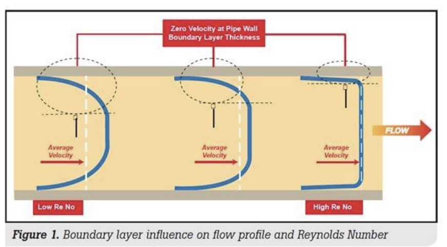
Flow in Pipe

• As Reynolds number increases beyond transition average flow profile goes from parabolic to closer to plug flow

  • Laminar boundary layer near the wall – Gets thinner as the Reynolds number increases

  • Thickness of boundary layer also influenced by surface roughness

Flow in Pipes - The Engineering Approach

• Fanning Friction factor:

  • Ratio of shear stress exerted on the fluid to its kinetic energy:

\[ f = \frac{\tau}{\rho \frac{v^2}{2}} \]

• For fully developed flow the shear stress on the wall must balance the pressure drop:

\[ \Delta P \pi R^2 = \tau 2 \pi R L \]

• Combine to give Fanning friction factor:

\[ f = \frac{\Delta P R}{L \rho v^2} \]

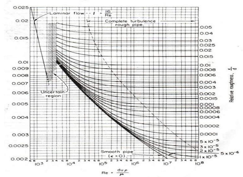
• Friction factor is a function of Reynolds Number and pipe roughness:

  • For laminar flow \( f = \frac{16}{re} \)

  • For turbulent flow empirical relationships or charts are used

Note that that Moody friction factor is often used instead of the Fanning friction factor, but it is simply 4 times larger

Example

• A horizontal pipe needs to have water flow through it at 0.1m3 /s

  • 𝜇 = 0.001 𝑃𝑎. 𝑠

  • 𝜌 = 1000 𝑘𝑔/𝑚3

• The pipe has a diameter of 30cm and can be assumed to be smooth

• If the pipe is 100m long, what pressure drop is required?

Flow given a Pressure Drop

• More complex to calculate unless laminar

Calculation tactic:

1. Guess a fluid velocity

2. Calculate Reynolds number

3. Look up the friction factor

4. Use the specified pressure drop to calculate a new fluid velocity based on the friction factor

5. Repeat from step 2 until sufficiently converged

Example

• If we halve the pressure drop calculated in the previous example, what will the new flowrate be?

Modelling Other Turbulent Flows

• Pipe flow is a very special case for which lots of experimental data is available

  • Can use empirical relationships to accurately predict behaviour What about turbulent flow in more complex geometries?

• Can readily rely on empirical data, especially if we want to use modelling for design

• We need to be able to understand and model turbulence

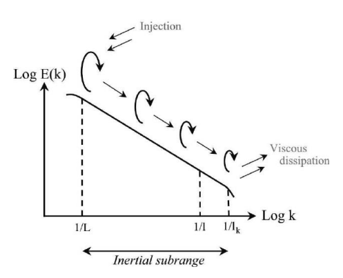
What Happens in Turbulent FLow?

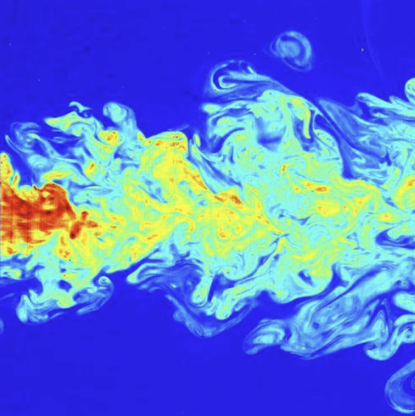
• At high Reynolds numbers large scale flow structures and instabilities will develop smaller scale perturbations

• This cascade of larger perturbations generating smaller flow structures will continue down until the flow structures are small enough that viscosity can “win”

  • The Kolmogorov length scale

• At this finest level the energy in the flow is dissipated as heat via the viscosity

Direct Numerical Simulation (DNS)

• Solve Navier-Stokes equation with enough resolution to resolve all the eddies down to their laminar cores

  • Very computationally expensive – prohibitively so for all but the lowest Reynolds numbers and smallest systems

• We can get a rough estimate of the resolution required based on Kolmogorov length scales and dimensional arguments

\[ \large \Delta x ~ \left( L \left( \frac{\mu}{\rho |v|} \right)^3 \right)^{\frac{1}{4}} \]

Water at 1 m/s in a 1 m channel would require a resolution of about 10 µm (about 1015 elements in a cubic box)!

Turbulence Modelling

• As DNS is only useable on a small range of problems, we need to model the effect of turbulence

• Turbulence dissipates more energy than the macroscopic strain rate would suggest

  • Need to calculate this extra dissipation

3 main approaches

• Simply increase the viscosity!

  • Trivial to do – often used in large scale simulations such as ocean modelling

• Assume that you can separate the turbulent and mean components of the flow

  • Reynold Average Navier Stokes (RANS) type models

  • We will look at the k-ε model as it is the most commonly used of this type

• Resolve as much as you can and then use a model for the bits you can’t resolve

  • Large Eddy Simulations (LES)

Both RANS and LES approaches involve the calculation of an additional turbulent viscosity that needs to be added to the underlying fluid viscosity

Mean and Fluctuating Flow Components

• Turbulent structures are typically embedded within macroscopic flow structures

• In analysing and modelling turbulence it is thus useful to distinguish between these flow components

• Assume that the flow at any point can be decomposed into a mean component and a fluctuating component:

\[ \large \mathbf{u} = \mathbf{U} + \mathbf{u}^{'} \]

where 𝐮 is the instantaneous velocity, 𝐔 is the average velocity and 𝐮′ is the fluctuating component of the velocity

RANS version of the Navier Stokes Equation

\[ \large \rho \frac{D \mathbf{u}}{Dt} = - \Delta p + \mu \nabla^2 \mathbf{u} + \rho \mathbf{g}\]

• Assume that there is a mean and fluctuating component of the velocity and pressure

  • Fluctuating component of pressure has no impact on final equation form

\[ \mathbf{u} = \mathbf{U} + \mathbf{u}^{'} \]

\[ p = P + p^{'} \]

• Substituting and applying the RANS averaging rules:

\[ \large \rho \frac{D \mathbf{U}}{Dt} = - \nabla P + \mu \nabla^2 \mathbf{U} + \rho \mathbf{g} - \rho \nabla \cdot \overline{ \mathbf{u}^{'} \mathbf{u}^{'} } \]

Reynolds Stress Tensor

• The averaged equation is similar to the original except for the inclusion of the divergence of a rank 2 tensor:

\[ \rho \nabla \cdot \overline{ \mathbf{u}^{'} \mathbf{u}^{'} } \]

• Known as the Reynolds Stress Tensor

\[\begin{split} \rho \overline{ \mathbf{u}^{'} \mathbf{u}^{'} } = \rho \left[ \begin{array} \\ \overline{u^{'} u^{'}} & \overline{u^{'} v^{'}} & \overline{u^{'} w^{'}} \\ \overline{u^{'} v^{'}} & \overline{v^{'} v^{'}} & \overline{v^{'} w^{'}} \\ \overline{u^{'} w^{'}} & \overline{v^{'} w^{'}} & \overline{w^{'} w^{'}} \\ \end{array} \right] \end{split}\]

\[ \mathbf{u}^{'} = \{ {u^{'},v^{'},w^{'}} \}\]

• Need to relate the Reynolds Stress Tensor to the mean flow

  • Know as the turbulence closure problem

  • No right way to do this, but some approximations are better than others

• The Reynolds Stress Tensor represents the transport of momentum due to the fluctuations in the flow

• In the standard Navier-Stokes equation the viscous stress term represents the “diffusion” of momentum

  • We can therefore think of Reynolds Stress Tensor in terms of a diffusion of momentum due to velocity fluctuations – a turbulent eddy viscosity

Turbulent Eddy Viscosity

• Write the Reynolds Stress Tensor in terms of the macroscopic strain rate:

\[ \overline{ \mathbf{u}^{'} \mathbf{u}^{'} } = -v_T ( \nabla \mathbf{U} +\nabla \mathbf{U}^T) \]

• This means that you can combine the liquid viscosity and the turbulent losses into a single effective viscosity:

  • In turbulence modelling it is often more convenient to use the kinematic viscosity

\[ v_{effective} = v + v_t \]

• We now need to calculate this turbulent eddy viscosity

Zero Equation Models

• The simplest type of turbulence model

  • Assume no explicit transport of turbulence

• Mainly based on dimensional arguments

  • \(l_0\) is a turbulent length scale, \(t_0\) is a turbulent time scale

\[ v_t = \frac{l^2_0}{t_0} \]

• Zero equation models are not very good in steady state RANS type models where the turbulent length scale is not well defined

  • Often adequate in LES models where the turbulent structures are resolved down to the grid resolution

    • Unresolved turbulent length scale similar to mesh resolution

    • Less transport of small scale turbulence before it is dissipated

• If we assume that we know the turbulent length scale, we still need the turbulent time scale from some macroscopic flow property

  • Two obvious candidates

    • Magnitude of the strain rate or magnitude of the vorticity

    • Both have units of inverse time

  • Based on strain rate – Smagorinsky mode

\[ \large v_T = ( C_s l_0)^2 |\mathbf{S}| \]

\[ \mathbf{S} = \frac{1}{2} (\nabla \mathbf{u} + \nabla \mathbf{u}^{T} ) \]

\(C_S\) is a tuneable constant. Typical values are 0.1-0.2

• Based on vorticity – Baldvin-Lomaz model

  • Less widely used than Smagorinsky – Use in modelling boundary layers

  • In boundary layers 𝑘 is a function of distance from the wall

\[ v_T = (k l_0)^2 |\mathbf{\omega}| \]

Two Equation Model

• We will revisit zero equation models in the context of LES

• For RANS modelling zero equation models are generally inadequate

• Need to consider the generation, transport and dissipation of turbulence

  • Two quantities can be used to model this

    • Turbulent kinetic energy - 𝑘

    • Turbulent dissipation rate - 𝜀

  • So called 𝑘 − 𝜀 turbulence model

    • Other models exist, but this is one of the most widely used and illustrates the idea

Turbulent Kinetic Energy - \(k\)

• The fluctuating components of the turbulence stores energy

  • This is known as the turbulent kinetic energy, 𝑘, which, per mass of fluid, can be written as follows:

\[ \large k = \frac{1}{2} \left( \overline{u^{'^{2}}} + \overline{v^{'^{2}}} + \overline{w^{'^{2}}} \right) \]

\[ \mathbf{u}^{'} = \{ u^{'},v^{'},w^{'} \} \]

• Note that the turbulent kinetic energy is therefore closely related to the Root Mean Square (RMS) of the velocity distribution

\[ u_{rms} = \sqrt{\overline{|\mathbf{u}^{'}|^2}} = \sqrt{\overline{|u^{'}|^2} + \overline{|v^{'}|^2} + \overline{|w^{'}|^2} }\]

• This turbulent kinetic energy is generated at the large scale and dissipated at the small scale

  • It can also be transported around the system by the mean flow

Turbulent Dissipation Rate - \(\varepsilon \)

• This is equal to the viscous losses associated with the fluctuating component of the velocity

  • I.e. the rate at which the turbulent kinetic energy is converted into thermal energy

\[ \large \varepsilon = v ~ \overline{ \mathbf{S}^{'} \cdot \mathbf{S}^{'} } \]

\[ \mathbf{S}^{'} = \frac{1}{2} ( \nabla \mathbf{u}^{'} + \nabla \mathbf{u}^{'T} ) \]

• While this is how the energy is dissipated, this equation is not directly useful as we do not know the fluctuation components (or their gradients)

Equations for \(k\) and \(\varepsilon\)

• Both the turbulent kinetic energy (𝑘) and the dissipation rate (𝜀) can be transported, generated and destroyed and are represented by a pair of coupled ODEs

  • Don’t worry too much about how these are derived – note, though, the additional complexity associated with modelling turbulence

\[\large \frac{\partial k}{\partial t} + \mathbf{U} \cdot \nabla k = \nabla \cdot \left( \frac{v_t}{\sigma_k} \nabla k \right) + 2 v_t \mathbf{S} \cdot \mathbf{S} - \varepsilon \]

\[ \mathbf{S} = \frac{1}{2} = ( \nabla \mathbf{U}^{'} + \nabla \mathbf{U}^{'T} ) \]

\[\large \frac{\partial \varepsilon}{\partial t} + \mathbf{U} \cdot \nabla k = \nabla \cdot \left( \frac{v_t}{\sigma_{\varepsilon}} \nabla \varepsilon \right) + C_{1 \varepsilon} \frac{\varepsilon}{k} \mathbf{S} \cdot \mathbf{S} - C_{2 \varepsilon} \frac{\varepsilon^2}{k} \]

\[ v_T = C_{\mu} \frac{k^2}{\varepsilon} \]

The semi-empirical constants are typically assigned the following values:

\[ C_{\mu} = 0.09, ~~ \sigma_k = 1.00, ~~ \sigma_{\varepsilon} = 1.30, ~~ C_{1 \varepsilon} = 1.44, ~~ C_{2, \varepsilon} = 1.92 \]

Boundaries in Turbulence Modelling

• At inlets both 𝑘 and 𝜀 need to be assigned values

  • If appropriate values are not assigned, long inlet regions will be required

• At walls 𝑘 is zero (no slip), but the transition typically occurs over a very narrow boundary layer

  • Typically need to model this boundary layer as it is usually computationally very expensive to explicitly resolve

Large Eddy Simulations - LES

• Transient simulations that resolve as much of the dynamics as possible

• Zero equation models are usually appropriate

  • No time averaging or smoothing of equations above the grid resolution

  • If unresolved resolution is small then the assumption of no turbulent transport between generation and dissipation is appropriate

• Can use Smagorinsky model with length scale as the grid resolution

\[ v_T = (C_s \Delta x)^2 |\mathbf{S}| \]

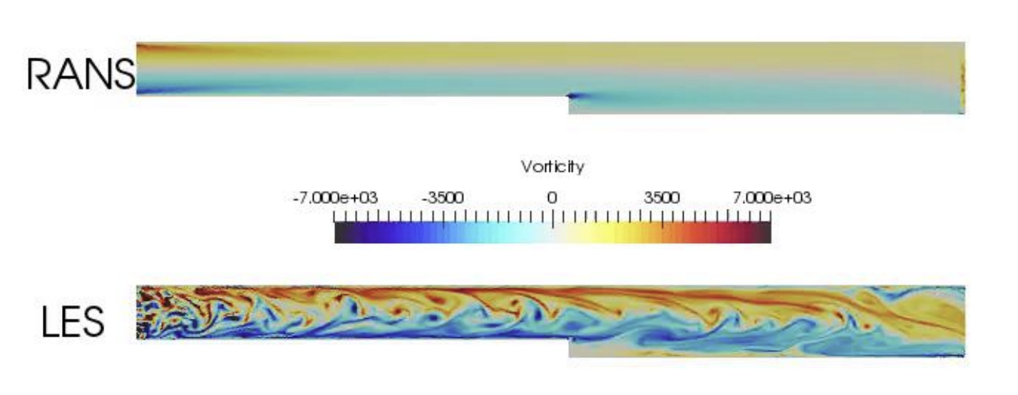
RANS vs LES

Other Rheologies

• Thus far we have only considered Newtonian rheology

  • Shear stress proportional to the strain rate

  • A good approximation for many fluids, importantly including water and virtually all gases

• Other Rheologies are possible

  • Shear stress a more complex function of strain rate

  • Can also be a function of strain history

    • Thixotropic fluids

Shear thinning

• Apparent viscosity decreases with strain rate

  • Quite common

    • Dense suspensions, emulsions, foams etc…

  • Sometimes called pseudo-plastic fluids

• Some physical origins:

  • Structures in the fluid can break down at high shears

    • E.g. some suspensions where particles can form flocs

  • Molecules align with or are extended in the shear direction

    • E.g. molten plastics

  • Particles in a fluid align with the flow and so move past one another more easily

Yield Stress

• An extreme example of shear thinning are materials with a yield stress

• Below a yield stress a material does not flow and acts like a solid

• Above the yield stress the material flows and acts like a liquid

• Quite common

  • It is really a matter of the size of the yield stress

  • Logical extension of plastic deformation in a solid

Shear thickening

• Apparent viscosity increases with strain rate

  • Much less common

    • Classic example is corn starch in water

• Some physical origins:

  • Structures in the fluid jam and can’t pass one another as easily at high strain rates

• Lots of current interest in shear-thickening fluids

  • Flexible protection and armouring

Modelling non-Newtonian Rheologies

• Need to incorporate these rheologies into the Navier-Stokes equation

  • Require a relationship between shear stress and strain rate tensors

• Often easier to incorporate rheology as an apparent viscosity that depends on strain rate

  • Note that in most solvers it is the velocity (and thus strain rate) that is assumed to be known

Power law fluid

• The simplest model for both shear thinning and shear thickening

  • The separation of the strain rate into two terms is so that stress tensor points in the correct direction

\[ \mathbf{\tau} = 2 k | 2 \mathbf{S} |^{n-1} \mathbf{S} \]

• if \(n=1\) this is Newtonian

• if \(n>1\) this is shear thickening

• if \(n<1\) this is shear thinning

\[ \mu_{eff} = k |2\mathbf{S}^{n-1}| \]

• If the velocity is in the y direction and only changes in the x direction

\[ \tau = k \frac{\partial u_y}{\partial x} \left| \frac{\partial u_y}{\partial x} \right|^{n-1} \]

Bingham Plastic

• The simplest type of yield behaviour is to assume that there is a yield stress followed by a linearly increasing stress with increasing strain rate

\[\large \text{if} ~ |\tau| > |\tau_0| ~ : ~~ \tau = (2 \mu_{\infty} |\mathbf{S}| + \tau_0 ) \frac{\mathbf{S}}{|\mathbf{S}|} \]

\[\large \text{if} ~ |\tau| < |\tau_0| ~ : ~~ \mathbf{S} = 0 \]

\[ \text{if} ~ |\tau| > |\tau_0| ~ : ~~ \mu_{eff} = 2 \mu_{\infty} + \frac{\tau_0}{|\mathbf{S}|} \]

\[ \text{if} ~ |\tau| < |\tau_0| ~ : ~~ \mu_{eff} = \infty \]

• If the velocity is in the y direction and only changes in the x direction

\[\large \text{if} ~ |\tau| > |\tau_0| ~ : ~~ \tau = sign \left( \frac{\partial u_y}{\partial x} \right) \left( k \left( \left| \frac{\partial u_y}{\partial x} \right| \right)^{n} +\tau_0 \right)\]

\[\large \text{if} ~ |\tau| < |\tau_0| ~ : ~~ \frac{\partial u_y}{\partial x} = 0 \]

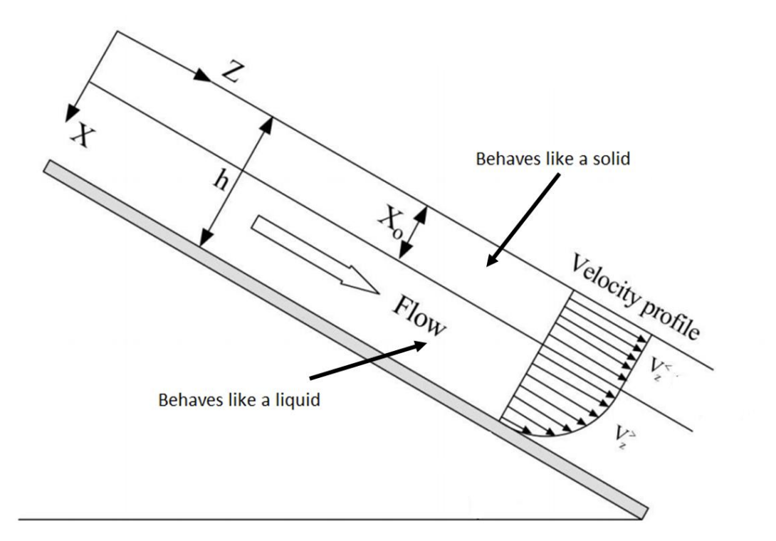
Free Surface Flow on an Inclined Plane

• This is the problem that we solved earlier for a Newtonian fluid

• Let us consider a Bingham plastic with a yield stress \(𝜏_0\)

Calculation :

• The shear stress distribution in this problem is the same as that for the Newtonian fluid and can be obtained in the same manner:

\[ \tau_{xz} = - \rho g \cos (\beta) x \]

Note that again 𝑥 is defined as the distance below the free surface

As the 𝑥𝑧 component is the only non-zero shear stress:

\[ \text{if} ~ |\tau_{xz}| > |\tau_0| ~ : ~~ \tau_{xz} = sign \left( \frac{d u_z}{d x} \right) \left( \mu_{\infty} \left| \frac{ d u_z}{d x} \right| +\tau_0 \right) \]

\[ \text{if} ~ |\tau_{xz}| < |\tau_0| ~ : ~~ \frac{d u_z}{d x} = 0 \]

• If we assume that the geometry is defined such that 𝜌𝑔cos 𝛽 is a positive number, then \(|𝜏_{𝑥𝑧}| = − 𝜏_{𝑥𝑧} \text{and} |\frac{du_z}{dx}| = -\frac{du_z}{dx} \) (note that if \(𝜏_{𝑥𝑧}\) was positive, which would have been the case if we had defined 𝑥 as being the distance above the bottom of the flow, then \(𝜏_{𝑥𝑧} = 𝜏_{𝑥𝑧} \text{and} |\frac{du_z}{dx}| = -\frac{du_z}{dx} \)

\[ \text{if} ~ -\tau_{xz} > \tau_0 ~ : ~~ \tau_{xz} = \left( \mu_{\infty} \left| \frac{ d u_z}{d x} \right| +\tau_0 \right) \]

\[ \text{if} ~ -\tau_{xz} < \tau_0 ~ : ~~ \frac{d u_z}{d x} = 0 \]

• We need to do this in two regions

  • A deep region when \(-𝜏_{𝑥𝑧} > 𝜏_0\) and a shallow region where \(-𝜏_{𝑥𝑧} < 𝜏_0\)

  • Let \(𝑥_0\) be the depth below the liquid surface of this transition:

\[ x_0 = \frac{\tau_0}{\rho g \cos(\beta)} \]

• In the deep region (\( x > x_0\)):

\[ -\mu_{\infty} \frac{d u_z}{dx} + \tau_0 = \rho g \cos(\beta) x \]

• Which can be integrated to give:

\[ u_z = \frac{-\rho g \cos(\beta)}{2 \mu_{\infty}} x^2 + \frac{\tau_0}{\mu_{\infty}} x + B \]

• B can be onbtained from no slip at the bottom ( \(v_z = 0 ~~ \text{at} ~~ x = h\))

\[ u_z = \frac{-\rho g \cos(\beta)}{2 \mu_{\infty}} (h^2 - x^2) - \frac{\tau_0}{\mu_{\infty}} (h - x) \]

• The velocity in the top portion is constant and can be obtained by setting \(x = x_0\):

\[ \text{if} ~ x > x_0: ~ u_z = \frac{-\rho g \cos(\beta)}{2 \mu_{\infty}} (h^2 - x^2_0) - \frac{\tau_0}{\mu_{\infty}} (h - x_0) \]

• Yielding following overall velocity profile:

\[\begin{split} u_z = \begin{cases} \frac{-\rho g \cos(\beta)}{2 \mu_{\infty}} (h^2 - x^2_0) - \frac{\tau_0}{\mu_{\infty}} (h - x_0) & \text{if }~~ x < x_0 \\ \frac{-\rho g \cos(\beta)}{2 \mu_{\infty}} (h^2 - x^2) - \frac{\tau_0}{\mu_{\infty}} ( h - x) & \text{if }~~ x > x_0 \\ \end{cases} \end{split}\]

Where: \(x_0 = \frac{\tau_0}{\rho g \cos(\beta)}\)

Bingham plastic velocity profile