1.3 Intro to Tensors#
Lecture 1.3
Saskia Goes, s.goes@imperial.ac.uk
Table of Contents#
Learning outcomes#
Be able to perform tensor operations (addition, multiplication) on Cartesian orthonormal bases
Be able to do basic tensor calculus (time and space derivatives, divergence, curl of a vector field) on these bases.
Understand differences/commonalities tensor and vector
Use index notation and Einstein convention
Tensors#
Tensors are a generalisation of vectors to more dimensions
Use when properties depend on direction in more than one way.
A physical quantity that is independent of coordinate system is used
Derives from the word tension (= stress)
Stress tensor is an example
Not just a multidimensional array
Further examples of the uses of tensors include: Stress, strain, and moment tensors. Electrostatics, electrodynamics, rotation, crystal properties
Tensor Rank#
Tensors describe properties that depend on direction
Tensor rank 0 - scalar - independent of direction
Tensor rank 1 - vector - depends on direction in 1 way
Tensor rank 2 - tensor - depends on direction in 2 ways
Notation #
Tensors as \(\mathbf{T}\)
Second order tensors wirtten as \(\bar{\bar{\mathbf{T}}}\) or \(\underline{\underline{\mathbf{T}}}\)
Index notation: \(T_{ij}\) where \(i,j=x,y,z\) or \(i,j=1,2,3\)
For higher order: \(T_{ijkl}\)
An Example Tensor#
Here is an example of a tensor, the gradient of velocity that depends on direction in two ways
Where each numerator, \(v_j\), is a component of velocity and each denominator \(x_i\) is the direction of the spatial variation, \(\frac{\partial v_j}{\partial x_i}\).
This tensor gradient definition is common in fluid dynamics
Note: some texts (including Lai et al., Reddy)
use a transposed definition:
Stress Tensor #
Body forces - depend on volume, e.g. gravity
Surface forces - depend on surface area, e.g. friction
Forces introduce a state of stress in a body, where stress is force per area
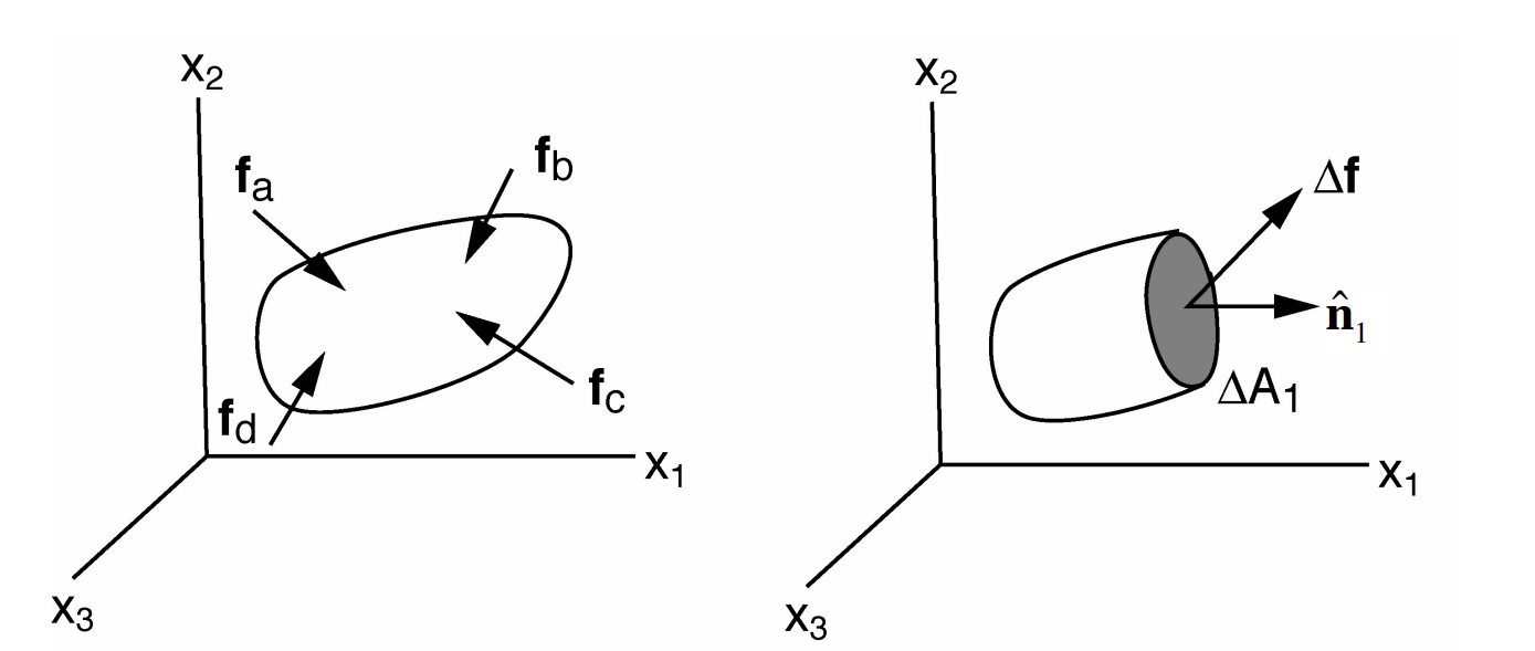
the \(\Delta\mathbf{f}\) necessary to maintain equilibrium depends on orientation of the plane on which stress is considered. The orientation of the plane can be described by the direction of it normal, unit vector \(\hat{\mathbf{n}}\)
e.g. on a plane with normal in \(x_1\) direction, \(\hat{\mathbf{n}}_1\), the traction, \(\mathbf{t_1}\) on the surface is defined as:
Nine components are needed to fully describe the stress in 3 dimensions on all possible planes.
Generalised stress tensor:
First index indicates orientation of plane
Second index indicates orientation of force
Distinction between tensor and its matrix #
Tensor – a physical quantity that is independent of coordinate system used
Matrix of a tensor – contains components of that tensor in a particular coordinate frame
You could test that indeed tensor addition and multiplication satisfy transformation laws
Tensor Operations #
Summation (Einstein) Convention #
When an index in a single term is a duplicate, dummy index, summation is implied without writing the summation symbol. An example is shown below:
An example with three terms is shown below:
The example below is invalid, as there are indices repeated more than twice
For more details see https://en.wikipedia.org/wiki/Einstein_notation
Notation Conventions #
Index notation - \(\alpha_{ij} x_i y_j = \sum_{i=1}^3 \sum_{j=1}^3 \alpha_{ij} x_i y_j\)
Matrix-vector notation - \(\mathbf{x^T A y} = (\begin{array} \\ x_1 & x_2 & x_3\end{array})\) \(\left[\begin{array} \\ \alpha_{11} & \alpha_{12} & \alpha_{13} \\ \alpha_{11} & \alpha_{12} & \alpha_{13} \\ \alpha_{11} & \alpha_{12} & \alpha_{13} \\ \end{array}\right]\) \(\left(\begin{array} \\ y_1 \\ y_2 \\ y_3\end{array}\right)\)
Other versions of index notation - \(x_i \alpha_{ij} y_j = \alpha_{ij} x_i y_j = \alpha_{ij} y_j x_i\)
Dummy vs Free Index #
\(i,k\) - dummy index: appears in duplicates and can be substituted without changing equation
\(j\) - free index, appears once in each term of the equation
Addition and Subtraction of Tensors#
\(\mathbf{W} = a\mathbf{T}+b\mathbf{S}\)
add each component: \(W_{ijkl} = aT_{ijkl} + bS_{ijkl}\)
\(\mathbf{T}\) and \(\mathbf{S}\) must have the same rank, dimension and units.
\(\mathbf{W}\) has takes the same rank, dimension and units as \(\mathbf{T}\) and \(\mathbf{S}\)
\(\mathbf{T}\) and \(\mathbf{S}\) are tensors, hence \(\mathbf{W}\) is a tensor. Tensor addition is commutative and associative.
This is the same as how vectors and matrices are added.
Multiplication of Tensors#
Inner product#
= dot product
\(\mathbf{W} = \mathbf{T \cdot S}\) involves contraction over one index: \(W_{ik} = T_{ij} S_{jk}\), as normal matrix and matrix-vector multiplication.
\(\mathbf{T}\) and \(\mathbf{S}\) can have different rank, but the same dimension.
rank of \(\mathbf{W} = \) rank of \(\mathbf{T}\) + rank of \(\mathbf{S} - 2\), dimensions as \(\mathbf{T}\) and \(\mathbf{S}\) units as product of units \(\mathbf{T}\) and \(\mathbf{S}\)
\(\mathbf{T}\) and \(\mathbf{S}\) are tensors, hence \(\mathbf{W}\) is a tensor.
Examples:
\(\lvert \mathbf{v} \rvert^2 = \mathbf{v \cdot v}\)
\(\bar{\bar{\mathbf{\sigma}}} = \bar{\bar{\bar{\bar{\mathbf{C}}}}}:\bar{\bar{\mathbf{\epsilon}}}\) or \(\sigma_{ij} = C_{ijkl} \epsilon_{kl}\) - Hooke’s Law
Tensor product#
= outer product = dyadic product \(\neq\) cross product
\(\mathbf{W} = \mathbf{TS}\) is often written as \(\mathbf{W} = \mathbf{T \otimes S}\)
No contraction: \(W_{ijkl} = T_{ij} S_{kl}\)
\(\mathbf{T}\) and \(\mathbf{S}\) can have different rank, but same dimension.
Rank of \(\mathbf{W}\) = rank of \(\mathbf{T}\) + rank of \(\mathbf{S}\), dimension as \(\mathbf{T}\) and \(\mathbf{S}\), units as product of units \(\mathbf{T}\) and \(\mathbf{S}\).
\(\mathbf{T}\) and \(\mathbf{S}\) are tensors, hence \(\mathbf{W}\) is a tensor.
Examples:
\(\mathbf{\nabla v}\) (gradient of a vector) \(\neq \mathbf{ \nabla \cdot v}\) (divergence)
remember that gradient is a vector \( \nabla = \left( \frac{\partial}{\partial x_1}, \frac{\partial}{\partial x_2}, \frac{\partial}{\partial x_3} \right)\)
For both multiplications#
Distributive: \(\mathbf{A(B+C) = AB + AC}\)
Associative: \(\mathbf{A(BC) = (AB)C}\)
Not commutative: \(\mathbf{TS \neq ST}\) and \(\mathbf{T \cdot S \neq S \cdot T}\)
However: \(\mathbf{T\cdot S = S^T \cdot T^T}\)
And: \(\mathbf{ab = (ba)^T)}\) but only for rank 2
Remember transpose: \(\mathbf{a \cdot T \cdot b = b \cdot T^T \cdot a} \longrightarrow T_{ji} = T_{ij}^T\)
Special tensor - The Kronecker delta#
\(\mathbf{\delta}_{ij} = \mathbf{\hat{e}}_i \cdot \mathbf{\hat{e}}_j\)
\(\mathbf{\delta}_{ij} = 1\) for \(i = j\), \(\mathbf{\delta}_{ij} = 0\) for \(i \neq j\)
In 3-D:
\(\mathbf{T \cdot \delta = T \cdot I = T}\) or \(T_{ij} \mathbf{\delta}_{jk} = T_{ik}\)
Isotropic tensors, invariant upon coordinate transformation:
scalars
\(\mathbf{0}\) vector
\(\delta_{ij}\)
\(\mathbf{\delta}\) is isotropic: \(\delta_{ij} = \delta_{ij}^{'}\) upon coordinate transformation can be used to write dot product: \(T_{ij} S_{jl} = T_{ij} S_{kl} \delta_{jk}\) can be used to write trace: \(A_{ii} = A_{ij} \delta_{ij}\).
Orthonormal transformation: \(\alpha_{ij} \alpha_{jk}^T = \delta_{ik}\)
Special tensor - Permutation symbol#
\(\epsilon_{ijk} = (\mathbf{\hat{e}}_i \times \mathbf{\hat{e}}_j) \cdot \mathbf{\hat{e}}_k\)
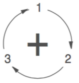
\(\epsilon_{ijk} = 1\) if \(i,j,k\) are an even permutation of 1,2,3
\(\epsilon_{ijk} = -1\) if \(i,j,k\) are an odd permutation of 1,2,3
\(\epsilon_{ijk} = 0\) for all other \(i,j,k\)
An even permutation follows the order 1 - 2 - 3, an odd permutation follows the order 1 - 3 - 2
Example:
\(\epsilon_{123} = \epsilon_{231} = \epsilon_{312} = 1\)
\(\epsilon_{213} = \epsilon_{321} = \epsilon_{132} = -1\)
\(\epsilon_{111} = \epsilon_{112} = \epsilon_{222} = ... = 0\)
Note that \(\epsilon_{ijk}a_ib_j\mathbf{\hat{e}}_k\), where \(\mathbf{\hat{e}}_k\) is the unit vector in \(k\)-th direction, is index notation for the cross product \(\mathbf{a \times b}\)
Useful identity: \(\epsilon_{ijm} \epsilon_{klm} = \delta_{ik} \delta_{jl} - \delta_{il} \delta_{jk}\)
Vector Derivatives - Curl#
Curl of a vector:
Some Tensor Calculus#
Gradient of a vector is a tensor:
Such that the change \(\mathbf{dv}\) in field \(\mathbf{v}\) is: \(\mathbf{dv} = \mathbf{dx \cdot \nabla v}\)
Divergence of a vector:
Trace of a tensor is the sum of diagonal elements
Divergence of a tensor:
Laplacian = div(grad f), where f is a scalar function:
Summary#
Vectors
– Addition, linear independence
– Orthonormal Cartesian bases, transformation
– Multiplication
– Derivatives, del, div, curl
Tensors
– Tensors, rank, stress tensor
– Index notation, summation convention
– Addition, multiplication
– Special tensors, \(\delta_{ij}\) and \(\epsilon_{ijk}\)
– Tensor calculus: gradient, divergence, curl, ..
Further reading/studying e.g:
– Reddy (2013): 2.2.1-2.2.3, 2.2.5, 2.2.6,2.4.1, 2.4.4, 2.4.5, 2.4.6, 2.4.8 (not co/contravariant)
– Lai, Rubin,Kremple (2010): 2.1-2.13, 2.16, 2.17, 2.27-2.32, 4.1-4.3
– Khan Academy – linear algebra, multivariate calculus
Try yourself#
For this part of the lecture, try \(\color{blue}{\text{Exercise 7}}\) and optional advanced \(\color{orange}{\text{Exercise 8}}\)
Try to finish in the afternoon workshop: \(\color{blue}{\text{Exercise 2, 3, 5, 6, 7, 9}}\)
Additional practise: \(\color{green}{\text{Exercise 1, 4}}\)
Advanced practise: \(\color{orange}{\text{Exercise 8, 10}}\)