6.1 Potential Flow

6.1 Potential Flow #

Lecture 6.1

Stephen Neethling, s.neethling@imperial.ac.uk

Learning outcomes #

Derive the potential flow equation
- Laplace’s equation for constant resistance
Be able to recognise a range of physical systems that obey potential flow
Show that the Navier-Stokes equation can be approximated as a potential flow under certain circumstances
- Including deriving a vorticity formulation for the Navier-Stokes equation
Demonstrate the stream function formulation for solving incompressible flow problems
- Demonstrate with potential flow problems
Demonstrate numerical solutions for Laplace’s equations

Do not alter this cell. LaTeX commands for frequently used terms.

\[\newcommand{\tensor}[1]{\underline{\underline{\mathbf{#1}}}}\]

\[\newcommand{\vector}[1]{\mathbf{#1}}\]

\[\newcommand{\ex}{\vector{\hat{e}}_1}\]

\[\newcommand{\ey}{\vector{\hat{e}}_2}\]

\[\newcommand{\ez}{\vector{\hat{e}}_3}\]

\[\newcommand{\x}{\vector{x}}\]

\[\newcommand{\v}{\vector{v}}\]

\[\newcommand{\u}{\vector{u}}\]

# Import packages for notebook here
import numpy
import matplotlib.pyplot as plt

%matplotlib inline

Potential Flow #

Potential flow is often used for the specific case of inviscid (zero viscosity) and incompressible fluid flow.

In this lecture, I will be using potential flow to describe a wider number of problems which can be modelled using Laplace’s equation.

We will also look at numerical solutions of Laplace’s equation. Analytical solutions do exist, but only in the form of infinite series.

Flow is proportional to the gradient of a potential:

\[ \large{\mathbf{v} = -k\nabla \phi} \]

Flow continuity holds:

\[ \large{\nabla \cdot \mathbf{v} = 0} \]

If the proportionality is constant this results in Laplace’s Equation:

\[ \large{\nabla^2 \phi = 0} \]

Good Approximations for Potential Flow #

One type of situation where potential is a good approximation is when the potential exerts a “force” on the quantity being observed, such as an electrical current or a fluid volume. The resistance to the flow is proportional to the flow-rate of the conserved quantity.

It is a good approximation for a number of systems:

Heat Flow
Electrical Current
Saturated flow in porous media

Flow in Porous Media #

This is used in a wide range of systems such as:

Packed bed catalytic reactors
Water flow in aquifers
Petroleum reservoirs
Porous electrodes in flow batteries and fuel cells

It is often characterised by a permeability, \(k\), with viscosity as a separate term in order to separate the porous media and the fluid effect:

\[ \large{\mathbf{v} = -\frac{k}{\mu} \nabla P} \]

Note that this velocity is the superficial velocity (volumetric flow rate per area of porous media) rather than the actual average velocity of the fluid. The porosity of the media is the factor by which the superficial velocity will be lower than the average fluid velocity.

However it does get more complicated for multi-phase flow in porous media due to the introduction of relative permeabilities that are a function of volume fraction of that phase in the pore space and capillarity (forces due to surface tension) can further complicate the situation.

Random Motion #

Random motion can also lead to potential flow

Diffusion is a good example. Thermal motion of molecules in a solvent leads to molecules of the solute being randomly nudged (Brownian motion). At the microscopic scale, heat flow follows a similar process as the kinetic energy of the particles is randomly transferred to neighbouring particles.

If particle motion is random, the number of particles leaving a small volume in a given time will be proportional to the number of particles in the volume. The number of particles entering will be proportional to the number of particles in the neighbouring regions. This will results in a net flow down a concentration gradient.

Diffusion through a random walk #

If we assume that Brownian motion causes a particle of the solute to take a random step of size \( \Delta x\) in time \( \Delta t\), this will result in the following macroscopic diffusion coefficient:

\[ \large{D = \frac{\Delta x^2}{2 \Delta t}} \]

\[ \Delta x \hspace{0.1cm} \text{is the Root Mean Square (RMS) of the step size if the step size varies} \]

The macroscopic flux can then be expressed as a function of the diffusion coefficient and the gradient of the concentration:

\[ \large{\mathbf{F} = -D \nabla C} \]

Implications of Potential Flow #

The flux is pure potential flow is always irrotational (curl of the vector is zero):

\[\begin{split} \large{\nabla \times \mathbf{v} = 0} \hspace{2cm} \nabla \times \mathbf{v} = \begin{pmatrix} \frac{\partial v_z}{\partial y} - \frac{\partial v_y}{\partial z} \\ \frac{\partial v_x}{\partial z} - \frac{\partial v_z}{\partial x} \\ \frac{\partial v_x}{\partial z} - \frac{\partial v_z}{\partial x} \\ \end{pmatrix} \end{split}\]

Try proving this

The reverse is also true: Irrotational flows can be written as potential flows.

Vorticity #

Potential flow implies irrotationality, which means that it has a vorticity:

\[ \large{\omega = \nabla \times \mathbf{v}} \]

Vorticity, \(\omega\), is a measure of the rotation of the flow. However, this can be misleading - fluid that has a curving flow path can have zero vorticity while fluid going in a straight line can have a non-zero vorticity.

Vorticity is a measure of the rotation of a small parcel of fluid - if you put a small twig in the flow will it rotate? (the average path it follows is immaterial to the vorticity?)

In 3D flow, the axis of the rotation is in the direction that the vorticity vector points and the length of the vector is proportional to how fast it rotates.

Incompressible, Inviscid Flow #

Why is incompressible inviscid flow a potential flow problem?

You have already derived the Navier-Stokes equations (more detail on it later in the course). However, it is important to know what each term represents;

\[ \text{Momentum Balance:} \hspace{1cm} \large{\color{orange}{\rho \frac{\partial \mathbf{u}}{\partial t}} + \color{green}{\rho \mathbf{u} \cdot \nabla \mathbf{u}} = \color{blue}{- \nabla P} + \color{purple}{\mu \nabla^2 \mathbf{u}} + \color{red}{\rho g}} \]

\[ \color{orange}{\text{Rate of change of momentum}} \hspace{1cm} \color{green}{\text{Flow of momentum (inertial force)}} \hspace{1cm} \color{blue}{\text{Pressure}} \hspace{1cm} \color{purple}{\text{Viscous force}} \hspace{1cm} \color{red}{\text{Body force}} \]

\[\begin{split} \text{Incompressible Continuity} \hspace{1.5cm} \nabla \cdot \mathbf{u} = 0 \hspace{1.5cm} \mathbf{u} \cdot \nabla \mathbf{u} = (\mathbf{u} \cdot \nabla)\mathbf{u} = \mathbf{u} \cdot (\nabla \mathbf{u}) = \begin{pmatrix} u_x \frac{\partial u_x}{\partial x} + u_y \frac{\partial u_x}{\partial y} + u_z \frac{\partial u_x}{\partial z} \\ u_x \frac{\partial u_y}{\partial x} + u_y \frac{\partial u_y}{\partial y} + u_z \frac{\partial u_y}{\partial z} \\ u_x \frac{\partial u_z}{\partial x} + u_y \frac{\partial u_z}{\partial y} + u_z \frac{\partial u_z}{\partial z} \\ \end{pmatrix} \end{split}\]

We can obtain the vorticiy equation by taking the curl (\(\nabla \times\)) of the Navier-Stokes equation. Using \(\omega = \nabla \times \mathbf{u}\) as the variable for vorticity:

\[ \large{\frac{\partial \omega}{\partial t}} + \mathbf{u} \cdot \nabla \omega = (\omega \cdot \nabla)\mathbf{u} + \frac{\mu}{\rho} \nabla^2 \omega + \nabla \times g \]

Note that the pressure does not appear in this equation if the density is constant (incompressible flow) as the curl of the gradient of a scalar is always zero.

Try and derive this. You will also need to use the incompressible assumption: \(\nabla \cdot \mathbf{u} = 0\)

Additionally the following identities useful:

\( \nabla \times (\mathbf{a} + \mathbf{b}) = \nabla \times \mathbf{a} + \nabla \times \mathbf{b} \)

\( \nabla \times (\nabla^2 \mathbf{a}) = \nabla^2 (\nabla \times \mathbf{a}) \)

\( \nabla \times (\nabla a) = 0 \)

\( \nabla \times \frac{\partial \mathbf{a}}{\partial t} = \frac{\partial}{\partial t} (\nabla \times \mathbf{a}) \)

\( \nabla \times (\mathbf{a} \times \mathbf{b}) = -\mathbf{b} (\nabla \cdot \mathbf{a}) + (\mathbf{b} \cdot \nabla)\mathbf{a} - (\mathbf{a} \cdot \nabla) \mathbf{b} \)

\( (\mathbf{u} \cdot \nabla) \mathbf{u} = \nabla \Bigl(\frac{1}{2}\mathbf{u} \cdot \mathbf{u}\Bigr) - \mathbf{u} \times \omega \)

This implies that:

\( \nabla \times ((\mathbf{u} \cdot \nabla)\mathbf{u}) = (\mathbf{u} \cdot \nabla)\omega + (\nabla \cdot \mathbf{u})\omega - (\omega \cdot \nabla)\mathbf{u} \)

Now try deriving the Navier-Stokes vorticity formulation

\[ \large{\frac{\partial \omega}{\partial t}} + \mathbf{u} \cdot \nabla \omega = (\omega \cdot \nabla)\mathbf{u} + \frac{\mu}{\rho} \nabla^2 \omega + \nabla \times g \]

If we further assume that the flow is inviscid (zero \(\mu\)) and that there is a constant (or conservative, \(\nabla \hspace{0.1cm} \times \hspace{0.1cm} \mathbf{g} \hspace {0.1cm} = \hspace{0.1cm} 0\)) body force:

\[ \large{\frac{\partial \boldsymbol{\omega}}{\partial t} + \mathbf{u} \cdot \nabla \boldsymbol{\omega} = (\boldsymbol{\omega} \cdot \nabla)\mathbf{u}} \]

The left-hand side of this equation represents the evolution of the vorticity of a parcel of a fluid. This implies that if the vorticity starts with a zero value it will remain zero for all position and all times.

If we therefore assume that our flow is initially irrotational (zero vorticity), then it will remain irrotational if it incompressible and inviscid.

Side note: Zero vorticity is also a solution to the equation with viscosity

\[ \large{\frac{\partial \boldsymbol{\omega}}{\partial t} + \mathbf{u} \cdot \nabla \boldsymbol{\omega} = (\boldsymbol{\omega} \cdot \nabla)\mathbf{u} + \frac{\mu}{\rho} \nabla^2 \boldsymbol{\omega}} \]

but it is incompatible with a shear stress at the boundaries. A shear stress at the boundary will generate vorticity at teh boundary. The viscous term will then cause the vorticity to “diffuse” into the interior.

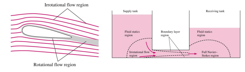
Because vorticity diffuses in boundaries, systems can have regions where potential flow is a good approximation and regions where it is not:

From our earlier discussion, irrotational flows can be described using a potential: \(\boldsymbol{u} = - \nabla \phi\)

As \(\nabla \cdot \boldsymbol{u} = 0\), this further implies that \(\nabla^2 \phi = 0\)

The potential described previously is NOT the same as the fluid pressure. To convert between them we need to use the Navier-Stokes Equation.

Navier-Stokes Equations for Incompressible Newtonian Flow:

\[ \large{\frac{\partial \mathbf{u}}{\partial t} + \mathbf{u \cdot u} = - \frac{\nabla P}{\rho} + \frac{\mu}{\rho} \nabla^2 \mathbf{u + g}} \]

\[ \large{\nabla \cdot \mathbf{u} = 0} \]

If we assume steady-state and inviscid, then the derivative term and viscosity term go to zero and we are left with:

\[ \large{(\mathbf{u} \cdot \nabla)\mathbf{u} = -\frac{\nabla P}{\rho} + \mathbf{g}} \]

\[ \large{\nabla \cdot \mathbf{u} = 0} \]

We can also use the identity from earlier:

\[ \large{(\mathbf{u} \cdot \nabla) \mathbf{u} = \nabla \Biggl(\frac{1}{2} \mathbf{u \cdot u} \Biggr) - \mathbf{u} \times \boldsymbol{\omega}} \]

Since \(\boldsymbol{\omega}\) is zero, this means that for an incompressible fluid (constant \(\rho\)):

\[ \large{\nabla \Biggl(\frac{1}{2} \mathbf{u \cdot u} \Biggr) = \nabla \Biggl( - \frac{P}{\rho} + \mathbf{g} \cdot \mathbf{x}\Biggr)} \]

Where x is the location vector.

Since \(\mathbf{u} = - \nabla \phi\) based on our previous derivation:

\[ \large{\nabla \Biggl( \frac{|\nabla \phi |^2}{2} \Biggr) = \nabla \Biggl( \frac{P}{\rho} - \mathbf{g \cdot x} \Biggr)} \]

This means that (less a constant of integration):

\[ \large{ P = \rho \Biggl( \frac{|\nabla \phi|^2}{2} + \mathbf{g \cdot x} \Biggr)} \]

Potential should be solved for first and then subsequently the pressure should be calculated even though they are not the same as one another.

Solving Potential Flow Problems #

While potential flow problems have a variety of physics that can be representedm the underlying equation that is being solved is always Laplace’s Equation.

\[ \large{\nabla^2 \phi = 0} \]

Since there is no time dependency in this equation and therefore its solution takes the form of a Boundary Value Problem. We therefore need to specify all boundaries.

Boundary Conditions #

Two linear boundary types are the specification of the potential at the boundary or the flux through the boundary. Potential specification is a Dirichelt Doundary condition in potential: \(\phi = f(\mathbf{x})\)

Flux specification is a Neumann boundary condition in potential. The condition specifies the values of the derivative applied at the boundary of the domain: \( \mathbf{v \cdot \hat{n}} = - k \nabla \phi \cdot \mathbf{\hat{n}} = F(\mathbf{x})\) where \(\mathbf{\hat{n}} \) is the unit normal to the boundary and \(F\) is the scalar flux through the boundary (in the direction of \(\mathbf{\hat{n}}\))

Stream Function Formulation #

Dirichlet boundary conditions are easier to implement than Neumann boundaries and typicallt result in quicker convergence when using a numerical solution scheme.

A stream function formulation allow flux boundary conditions to be specified using Dirichlet boundary conditions. However, it still doesn’t allow a mixture of potential and flux boundaries, which would still require a combination of Dirichlet and Neumann boundaries. We will solve problems of this type in the next lecture.

Stream Functions #

Stream functions can be used to represent 2D steady-state systems that exihibit continuity.

A stream function is a scalar field where flows follows a constant value of the function. In other words, a constant value of the stream functions represents a streamline.

Stream functions are just one way to solve potential flow problems and they only work in 2D. They can also be used in the analysis or the solution of other flow problems where continuity of glux holds.

This makes specifying flux conditions easier. For flux boundary conditions, the specification of a potential gradient at the boundary turns into the specification of a stream function value. (i.e turns a Neumann boundary condition, which is harder to solve, into a Dirichlet boundary conditon, which is easier to solve.)

Other properties of stream functions are:

Differences in the value of the stream function are equal to the flowrate of the conserved quantity between the streamlines represented by those stream function values.
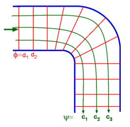
In potential flow problems, lines of constant value of the stream function are orthogonal to lines of constant value of the potential.

The stream function \(\psi\) is related to flux (volume flux is a velocity):

\[ \large{F_x = \frac{\partial \psi}{\partial y} \hspace{2cm} F_y = - \frac{\partial \psi}{\partial x}} \]

If this is substituted into the steady state continuity equation you can see that it is satisfied.

\[ \large{\nabla \cdot \mathbf{F} = 0} \hspace{1cm} \text{in 2D} \hspace{1cm} \frac{\partial F_x}{\partial x} + \frac{\partial F_y}{\partial y} = \frac{\partial^2 \psi}{\partial x \partial y} - \frac{\partial^2 \psi}{\partial x \partial y} = 0 \]

We also know that potential flow implies that there is zero vorticity. (\( \nabla \times \mathbf{F} = 0\))

Substituting the definitions of the fluxes into this equation results in Laplace’s equation (strictly speaking the curl is a vector, but in 2D there is only one non-zero component): \(\nabla^2 \psi = 0\)

Boundary Conditions #

Stream functions are useful if the boundaries are flux boundary conditions:

\[ \large{F_x = \frac{\partial \psi}{\partial y} \hspace{2cm} F_y = - \frac{\partial \psi}{\partial x}} \]

These definitions imply that the stream function is a constant value along a boundary for a zero flux condition and changes linearly for a constant flux. Other flux boundaries are readily solvable.

There are few points to note when calculating stream function values around a boundary:

The velocities in the system depend upon the gradient of hte stream function. Therefore, we have 1 degree of freedom when choosing the stream function values. Adding a constant to all the stream function values does not change the velocities calculated. You can therefore choose any value for the stream function at a single point on the boundary.
Values of the stream function must be continuous around the boundary. A discontinuity in the stream function is equivalent to an infinite flux. This will let you set the constants of integration obtained when deriving the boundary conditions.

Example #

A metal block 2m wide and 1m high is being heated from below and cooled on the left and right hand sides. The top boundary is thermally insulated.

You can assume that the block is insulated at the front and back making this a 2D problem. (It is 1m deep in this direction)

There is a constant heat flux into the bottom on the block of \(100 W/m^2\).

The heat splits evenly out of the left and right hand sides, with a constant flux through each of these sides.

What are the values of the stream function around the boundaries of the block?

Numerical Solutions to Laplace’s Equation #

Because these are solutions for steady-state systems, the solution takes the form of a Boundary Value Problem. Therefore, we need to specify conditions along all the boundaries and we need a discretised version of the governing equation to describe all the interior points as a function of their surrounding points.

Non-steady state problems take the form of Initial Value Problems. However we still need boundary conditions and require an initial value for all the locations in the system (hence initial value problem). The governing equation needs to not only describe the relationships between neighbouring points in space, but also in time.

Finite Difference Approximation #

Finite difference is the easiest way to approximate differentials on a grid. There are a number of ways in which first derivatives can be approximated on a grid, three of which are:

Central Difference: \(\hspace{1cm} \large{\Bigl( \frac{\partial u}{\partial x} \Bigr)_i \approx \frac{ u_{i + 1} \hspace{0.1cm} - \hspace{0.1cm} u_{i - 1} }{ 2 \Delta x}} \hspace{1cm}\) \( \text{2nd order accurate} \)
Forward Difference: \(\hspace{1cm} \large{\Bigl( \frac{\partial u}{\partial x} \Bigr)_i \approx \frac{ u_{i + 1} \hspace{0.1cm} - \hspace{0.1cm} u_{i} }{ \Delta x}} \hspace{1cm}\) \( \text{1st order accurate} \)
Backward Difference: \(\hspace{1cm} \large{\Bigl( \frac{\partial u}{\partial x} \Bigr)_i \approx \frac{ u_{i} \hspace{0.1cm} - \hspace{0.1cm} u_{i - 1} }{ \Delta x}} \hspace{1cm}\) \( \text{1st order accurate} \)

2nd order derivatives can also be approximated

\( \large{ \Bigl( \frac{\partial^2 u}{\partial x^2}} \Bigr)_i \approx \frac{u_{i + 1} - 2u_i + u_{i - 1}}{\Delta x^2} \)

Finite Difference Approximation of a Linear 2nd Order PDEs #

Using finite difference approximations, any 2D steady state linear 2nd order PDE can be approximated as follows:

\[ a_{i,j} \hspace{0.1cm} u_{i + 1,j} + b_{i,j} \hspace{0.1cm} u_{i - 1,j} + c_{i,j} \hspace{0.1cm} u_{i,j + 1} + d_{i,j} \hspace{0.1cm} u_{i,j - 1} + e_{i,j} \hspace{0.1cm} u_{i,j} = f_{i,j} \]

The prefactors a, b, c, d, e and f are matrices (i.e functions of position) in the general case, since the linear coefficients in the PDE can also be functions of position.

Approximating Laplace’s Equation #

\[ \nabla^2 \psi = \frac{\partial^2 \psi}{\partial x^2} + \frac{\partial^2 \psi}{\partial y^2} = 0 \]

Using our earlier approximations for the 2nd derivatives and with \(x = x_0 + i \Delta x\) and \(y = y_0 + j \Delta y\) as the difference for the grid:

\[ \nabla^2 \psi \approx \frac{\psi_{i + 1, j} - 2\psi_{i,j} + \psi_{i - 1, j}}{\Delta x^2} + \frac{\psi_{i, j + 1} - 2\psi_{i,j} + \psi_{i, j - 1}}{\Delta y^2} = 0 \]

If we further assume that the grid is square (\(\Delta x = \Delta y\)), then we need to solve the following approximation:

\[ \psi_{i + 1,j} + \psi_{i - 1,j} + \psi_{i, j + 1} + \psi{i, j - 1} - 4\psi_{i,j} = 0 \]

Using the form on the previous page: \(a = b = c = d = 1, e = -4, f = 0\)

Iterative and Inversion Methods #

\[ a_{i,j} \hspace{0.1cm} u_{i + 1,j} + b_{i,j} \hspace{0.1cm} u_{i - 1,j} + c_{i,j} \hspace{0.1cm} u_{i,j + 1} + d_{i,j} \hspace{0.1cm} u_{i,j - 1} + e_{i,j} \hspace{0.1cm} u_{i,j} = f_{i,j} \]

Since there is one of the above equations for each point in the solution grid, the problem takes the form of a set of coupled linear equations. There are therefore two main approaches that can be used:

Direct matrix solution or Inversion: This method can reach the solution in one step, however “stiff” problems (matrices with determinant close to zero, usually in problems with strong convective terms) can result in near singular matrices which give rise to problems with numerical precision.
Iterative methods: This method iteratively approaches the solution using a number of steps, each (hopefully) close to the solution than the previous one. This can be easier to implement and improved convergence speed often requires more complexity in the solution. Generally, it also has lower memory requirements than inversion techniques.

Iterative Methods #

Iterative methods work by successfully by successively reducing the error in the solution. The error we use is residual, which is the error in the approximation of the differential equation.

As we don’t know the final solution as a priori, we can’t use the error in the dependent variable. Equivalently, we could also use the change in the dependent variable with each iteration as a stopping criterion.

The residual at point \(i, j\) is:

\[ \xi_{i,j} = a_{i,j} \hspace{0.1cm} u_{i + 1,j} + b_{i,j} \hspace{0.1cm} u_{i - 1,j} + c_{i,j} \hspace{0.1cm} u_{i,j + 1} + d_{i,j} \hspace{0.1cm} u_{i,j - 1} + e_{i,j} \hspace{0.1cm} u_{i,j} - f_{i,j} \]

with iterations continuing until the residual drops below a certain value. For example, continue iterations until \( \large{\frac{\Sigma \Sigma |\xi_{i,j}|}{\Sigma \Sigma |e_{i,j} u_{i,j}|}} \) \(< \text{tolerance}\).

Jacobi Method #

From the finite difference approximation:

\[ a_{i,j} \hspace{0.1cm} u_{i + 1,j} + b_{i,j} \hspace{0.1cm} u_{i - 1,j} + c_{i,j} \hspace{0.1cm} u_{i,j + 1} + d_{i,j} \hspace{0.1cm} u_{i,j - 1} + e_{i,j} \hspace{0.1cm} u_{i,j} = f_{i,j} \]

We can rearrange this to set the midpoint value as a function of the neighbouring values:

\[ u_{i,j} = \frac{f_{i,j} - (a_{i,j} \hspace{0.1cm} u_{i + 1,j} + b_{i,j} \hspace{0.1cm} u_{i - 1,j} + c_{i,j} \hspace{0.1cm} u_{i,j + 1} + d_{i,j} \hspace{0.1cm} u_{i,j - 1} + e_{i,j} \hspace{0.1cm} u_{i,j}) }{e_{i,j}} \]

We can use this as the basis for an iterative solution:

\[ \large{u_{i,j}^{new}} = \frac{ f_{i,j} - (a_{i,j} \hspace{0.1cm} u_{i + 1,j}^{old} + b_{i,j} \hspace{0.1cm} u_{i - 1,j}^{old} + c_{i,j} \hspace{0.1cm} u_{i,j + 1}^{old} + d_{i,j} \hspace{0.1cm} u_{i,j - 1}^{old})}{e_{i,j}} \]

Steps in solving this problem #

Derive boundary conditions/values for each location on the boundary - We will use the Dirchlet boundary conditions in this example. We will therefore need the value of stream function at each point on thge edge of the grid.
Discretise the governing equation - We have already done this for Laplace’s Equation.
Give an initial guess for the stream function value at every point inside the grid - A good guess can be critical for the convergence of some systems, but it is not very important here as solutions of Laplace’s equation with Dirichlet boundary conditions converges quickly.
Implement the iterative solver - Calculate a new guess for the grid values based on the previous guess. Repeat until the residual (or change in the dependent variable) is sufficiently small.

Systems with more Complex Boundaries #

Thus far we have only considered problems with Dirichlet boundary conditions. (Values of the dependent variable specified along the boundary)

These are easier to solve numerically and have better convergence behaviour than Neumann and other more complex boundary conditions. It also makes analytical solutions tractable.

When solving numerically using SOR, the more complex boundary conditions will require that the points on the boundary are included in the iteration.

Neumann Boundary Conditions #

This boundary condition is often found in potential flow problems. For example, if the flux through the boundary is specified and the potential is the dependent variable.

\[ \large{F_{in} = - k\nabla \phi \cdot \mathbf{\hat{n}}} \]

Where \(F_{in}\) is the flux in through the boundary and the unit normal points into the domain.

A no flux boundary condition in potential flow is thus a zero gradient, which is a special case of the Neumann boundary condition.

Finite Difference Approximation of a Neumann Boundary #

As the point being considered by us is, by definition, on the edge of the valid domain, the central difference method can’t be used. Whether a forward or backward approximation is used depends on which side of the domain the boundary is.

For example, if the forward difference is in the x-direction on the left hand boundary and backward difference on the right hand boundary and similarly, in the y-direction a forward difference needs to be used in the bottom boundary and a backwards difference on the top boundary.

If the finite difference approximation is expressed as follows:

\[ a_{i,j} \hspace{0.1cm} u_{i + 1,j} + b_{i,j} \hspace{0.1cm} u_{i - 1,j} + c_{i,j} \hspace{0.1cm} u_{i,j + 1} + d_{i,j} \hspace{0.1cm} u_{i,j - 1} + e_{i,j} \hspace{0.1cm} u_{i,j} = f_{i,j} \]

and \(x_0, y_0\) is in the bottom left hand corner then:

Vertical Boundaries: \(\large{\frac{\partial u}{\partial x}}\) \( = g(y)\)

For the left hand boundary: \(a_{i, j} = 1, \hspace{0.1cm} b_{i, j} = c_{i, j} = d_{i, j} = 0, \hspace{0.1cm} e_{i,j} = -1 \hspace{0.5cm} f_{i,j} = \Delta x \hspace{0.1cm} g(y_j)\)
For the right hand boundary: \(b_{i, j} = -1, \hspace{0.1cm} a_{i, j} = c_{i, j} = d_{i, j} = 0, \hspace{0.1cm} e_{i,j} = 1 \hspace{0.5cm} f_{i,j} = \Delta x \hspace{0.1cm} g(y_j)\)

Horizontal Boundaries: \(\large{\frac{\partial u}{\partial y}}\) \(= g(x)\)

For the bottom boundary: \(c_{i, j} = 1, \hspace{0.1cm} a_{i, j} = b_{i, j} = d_{i, j} = 0, \hspace{0.1cm} e_{i,j} = -1 \hspace{0.5cm} f_{i,j} = \Delta y \hspace{0.1cm} g(x_i)\)
For the top boundary: \(d_{i, j} = -1, \hspace{0.1cm} a_{i, j} = b_{i, j} = c_{i, j} = 0, \hspace{0.1cm} e_{i,j} = 1 \hspace{0.5cm} f_{i,j} = \Delta y \hspace{0.1cm} g(x_i)\)

Robin Boundary Condition #

The third type of linear PDE boundary condition is the Robin boundary condition. This condition is a linear conmbination of Dirichlet and Neumann boundary condition.

\[ \nabla u \cdot \hat{n} + g(x,y) u = h(x, y) \]

This means that:

For a vertical boundary: \(\hspace{1cm} \large{\frac{\partial u}{\partial x}}\) \( + \hspace{0.1cm} g(y) u = h(y)\)
For a horizontal boundary: \(\hspace{1cm} \large{\frac{\partial u}{\partial y}}\) \( + \hspace{0.1cm} g(x) u = h(x)\)

Finite Difference Approximation of a Robin Boundary #

Again using the following form for the approximation:

\[ a_{i,j} \hspace{0.1cm} u_{i + 1,j} + b_{i,j} \hspace{0.1cm} u_{i - 1,j} + c_{i,j} \hspace{0.1cm} u_{i,j + 1} + d_{i,j} \hspace{0.1cm} u_{i,j - 1} + e_{i,j} \hspace{0.1cm} u_{i,j} = f_{i,j} \]

Vertical Boundaries: \(\large{\frac{\partial u}{\partial x}}\) \(+ \hspace{0.1cm} g(y) u = h(y)\)

For the left hand boundary: \(a_{i, j} = 1, \hspace{0.1cm} b_{i, j} = c_{i, j} = d_{i, j} = 0, \hspace{0.1cm} e_{i,j} = -1 + \Delta x \hspace{0.1cm} g(y_j) \hspace{0.5cm} f_{i,j} = \Delta x \hspace{0.1cm} h(y_j)\)
For the right hand boundary: \(b_{i, j} = -1, \hspace{0.1cm} a_{i, j} = c_{i, j} = d_{i, j} = 0, \hspace{0.1cm} e_{i,j} = 1 + \Delta x \hspace{0.1cm} g(y_j) \hspace{0.5cm} f_{i,j} = \Delta x \hspace{0.1cm} h(y_j)\)

Horizontal Boundaries: \(\large{\frac{\partial u}{\partial y}}\) \(+ \hspace{0.1cm} g(x) u = h(x)\)

For the bottom boundary: \(c_{i, j} = 1, \hspace{0.1cm} a_{i, j} = b_{i, j} = d_{i, j} = 0, \hspace{0.1cm} e_{i,j} = -1 + \Delta y \hspace{0.1cm} g(x_j) \hspace{0.5cm} f_{i,j} = \Delta y \hspace{0.1cm} h(x_i)\)
For the top boundary: \(d_{i, j} = -1, \hspace{0.1cm} a_{i, j} = b_{i, j} = c_{i, j} = 0, \hspace{0.1cm} e_{i,j} = 1 + \Delta y \hspace{0.1cm} g(x_j)\hspace{0.5cm} f_{i,j} = \Delta y \hspace{0.1cm} h(x_i)\)

Where do Robin Boundary Conditions Arise #

Robin boundary condtions are encountered in convective-diffusive problems.

Convective-diffusive problems are ones in which a flux is proportional to the sum of a zero order (convective) term and a 1st order diffusive term. Note that when substituted into a continuity equation, the convective term becomes 1st order and the diffusive term 2nd order. A flux with a convective and diffusive component takes the following form:

\[ \mathbf{F} = \mathbf{v} u - D \nabla u \]

where \(\mathbf{F}\) is the flux of \(u\). \(\mathbf{v}\) is the convective velocity vector and \(D\) is the diffusion coefficient.

If the flux through a boundary is \(F_{in}\) and \(\mathbf{\hat{n}}\) is the unit normal to the boundary pointing into the domain, then the flux boundary condition for a convective diffusive problem is:

\[ \large{F_{in} = (\mathbf{v \cdot \hat{n}})u - D \nabla u \cdot \mathbf{\hat{n}}} \]

This thus takes the form of the Robin boundary condition.