Exercises

Learning outcomes

At the end of this session, you should be able to:

1. Use material and spatial descriptions of variables and their time derivatives.

2. Compute infinitesimal strain (strain rate) tensor given a displacement (velocity) field.

3. Interpret the different components of the infinitesimal strain (rate) tensor

Table of Contents

# Import packages for notebook here
import numpy as np
import matplotlib.pyplot as plt

%matplotlib inline

Do not alter this cell. LaTeX commands for frequently used terms.

\[\newcommand{\tensor}[1]{\underline{\underline{\mathbf{#1}}}}\]

\[\newcommand{\vector}[1]{\mathbf{#1}}\]

\[\newcommand{\matrix}[1]{\mathbf{#1}}\]

\[\newcommand{\det}[1]{\mathrm{det}\left(#1\right)}\]

\[\newcommand{\ex}{\vector{\hat{e}}_1}\]

\[\newcommand{\ey}{\vector{\hat{e}}_2}\]

\[\newcommand{\ez}{\vector{\hat{e}}_3}\]

\[\newcommand{\nhat}{\vector{\hat{n}}}\]

\[\newcommand{\ehat}{\vector{\hat{e}}}\]

\[\newcommand{\xhat}{\vector{\hat{x}}}\]

\[\newcommand{\x}{\vector{x}}\]

\[\newcommand{\v}{\vector{v}}\]

\[\newcommand{\u}{\vector{u}}\]

Here we define a few functions that will be helpful in this notebook there’s no need to understand these now, but you may like to look at these later if you want to extend the notebook or tackle the extension exercises.

# Make a position grid fine enough to represent velocities as a smooth field.
def init_grid(Lx=10., dx=None, Ly=10., dy=None):

    # Use 100 grid points if dx not specified
    if dx is None:
        dx = Lx/100.
    if dy is None:
        dy = Ly/100.
    
    # Construct the grid
    nx = int(Lx/dx)
    xx = np.linspace(0, Lx, nx)
    ny = int(Lx/dx)
    yy = np.linspace(0, Ly, ny)
    X, Y = np.meshgrid(xx, yy)
    
    return X, Y

# Define the initial positions of a set of tracer particles to show motion/deformation
# Construct two 2D numpy arrays, one for each coordinate direction. The first dimension
# is the particle number; the second is the time level. . .
def tracers(p0=[[0.5, 0.5], [1.5, 0.5], [1.5, 1.5], [0.5, 1.5], [0.5, 0.5]], nt=11):
    
    # Create arrays
    px = np.zeros((len(p0), nt))
    py = np.zeros_like(px)

    # Initialise with specified initial coordinates.
    for p, i in zip(p0, range(len(p0))):
        px[i,:] = p[0]
        py[i,:] = p[1]
        
    return px, py

# Define a function for plotting 2D tensor components as scalar fields. . .
def plot_2D_tensor_field(X, Y, exx, exy, eyx, eyy, cmin=0., cmax=4., field='displ'):
    
    # same colour scale for gradients, strain components, divergence and curl
    cc = np.linspace(cmin, cmax, 21)
    
    # Define colormap based on range
    # https://matplotlib.org/stable/tutorials/colors/colormaps.html
    if (cmin < 0.):
        # Divergent colour scale for negative and positive fields
        plt.set_cmap("bwr")
    else:
        # Perceptually uniform sequential colormap for positive fields
        plt.set_cmap("viridis")

    # Plot displacement gradients
    fig = plt.figure(figsize=(7,7))
    ax11 = plt.subplot(2,2,1,aspect='equal')
    ax11.contourf(X, Y, exx, cc)
    ax11.set(ylabel='y')
    ax12 = plt.subplot(2,2,2,aspect='equal')
    ax12.contourf(X, Y, exy, cc)
    ax21 = plt.subplot(2,2,3,aspect='equal')
    ax21.contourf(X, Y, eyx, cc)
    ax21.set(xlabel='x', ylabel='y')
    ax22 = plt.subplot(2,2,4,aspect='equal')
    dyy = ax22.contourf(X, Y, eyy, cc)
    ax22.set(xlabel='x')

    if field == 'displ':
        fig.suptitle("displacement gradients (transpose)")
        ax11.set_title('$\partial u_x/\partial x$')
        ax12.set_title('$\partial u_y/\partial x$')
        ax21.set_title('$\partial u_x/\partial y$')
        ax22.set_title('$\partial u_y/\partial y$')
    elif field == 'strain':
        fig.suptitle("strain tensor")
        ax11.set_title('$E_{xx}$')
        ax12.set_title('$E_{xy}$')
        ax21.set_title('$E_{yx}$')
        ax22.set_title('$E_{yy}$')
    elif field == 'rotation':
        fig.suptitle("rotation tensor")
        ax11.set_title('$\omega_{xx}$')
        ax12.set_title('$\omega_{xy}$')
        ax21.set_title('$\omega_{yx}$')
        ax22.set_title('$\omega_{yy}$')
    elif field == 'vorticity':
        fig.suptitle("vorticity tensor")
        ax11.set_title('$W_{xx}$')
        ax12.set_title('$W_{xy}$')
        ax21.set_title('$W_{yx}$')
        ax22.set_title('$W_{yy}$')
    elif field == 'velocity':
        fig.suptitle("velocity gradients (transpose)")
        ax11.set_title('$\partial v_x/\partial x$')
        ax12.set_title('$\partial v_y/\partial x$')
        ax21.set_title('$\partial v_x/\partial y$')
        ax22.set_title('$\partial v_y/\partial y$')
    elif field == 'strainrate':
        fig.suptitle("strainrate tensor")
        ax11.set_title('$D_{xx}$')
        ax12.set_title('$D_{xy}$')
        ax21.set_title('$D_{yx}$')
        ax22.set_title('$D_{yy}$')
         
    plt.tight_layout()

    #set global colorbar
    cb_ax = fig.add_axes([1.0, 0.1, 0.05, 0.8])
    cbar = fig.colorbar(dyy, cax=cb_ax)
    plt.set_cmap("viridis")

Material vs spatial descriptions

In the lecture we introduced two alternative ways in which motion (flow or deformation) can be described: the material (Lagrangian) description or the spatial (Eulerian) description.

As an example, we considered the spatial description of a 2D velocity field given by:

\[v_i=\frac{kx_i}{(1+kt)},\]

where:

• \(v_i\) is the ith component of velocity,

• \(k\) is a constant,

• \(x_i\) is the ith component of the position vector,

• \(t\) is time.

We then showed how to define the spatial description of acceleration in this case. We then went on to derive the corresponding material description of the displacement (path lines), velocity and acceleration of a particle in the flow.

Spatial field

Let’s visualise what we did using Python. We start by defining the spatial description of our velocity field as a function of \(x\) (\(x_1\)), \(y\) (\(x_2\)) and \(t\).

# Define the spatial description of a 2D velocity field as a function of x, y and time.
# You can modify this to consider different spatial velocity functions. . . 
def velocity_spatial(x, y, t, k=1):
    return k*x/(1.+k*t), k*y/(1.+k*t)

Next we initialise a grid, time array, velocity arrays and tracer arrays

# Define a spatial grid with 100 x 100 points. . .
X, Y = init_grid(Lx=5., Ly=5.)

# Choose a time discretisation fine enough for integrating particle paths 
# with enough precision to reproduce the analytical solution discussed in the lecture.
dt = 0.05
tt = np.arange(0, 2 + dt, dt)
nt = tt.size

# Define three tracers to trace the pathlines
px, py = tracers(p0=[[0.8, 0.2], [0.8, 0.8], [0.8, 1.4]], nt=nt)

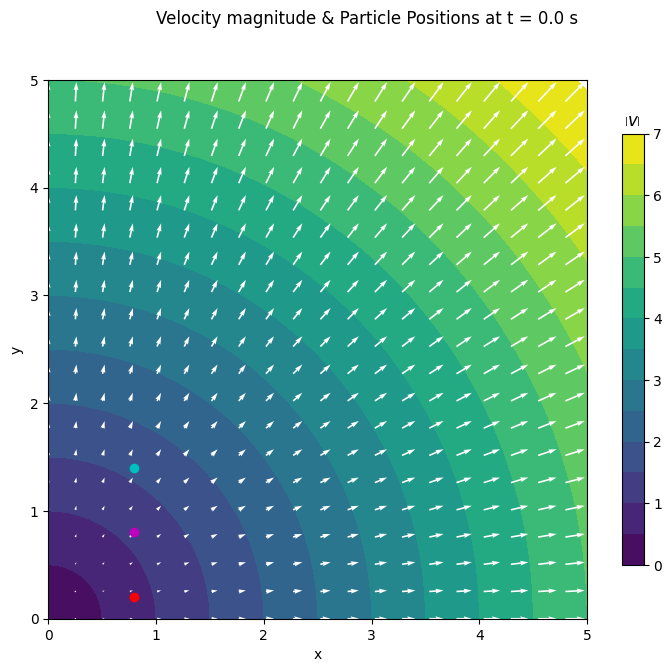
We can now plot the velocity vector field, the velocity magnitude scalar field and our particle positions at the intial time, 𝑡=0.

# Visualise the velocity field at time zero

# Define velocity vector field and velocity magnitude scalar field
k=1
vx, vy = velocity_spatial(X, Y, 0., k=k)
vmag = np.sqrt(vx**2 + vy**2)

# Plot the velocity field at time zero
plt.figure(figsize=(9,7))
plt.subplot(aspect='equal')
plt.suptitle("Velocity magnitude & Particle Positions at t = %1.1f s" % tt[0])
plt.xlabel('x')
plt.ylabel('y')

# Define a sensible fixed colorscale
cc = np.arange(0, 7.5, 0.5)
cl = np.arange(0, 8, 1)

# Contour plot of velocity magnitude
c = plt.contourf(X, Y, vmag, cc)
cbar = plt.colorbar(c, shrink=0.8, ticks=cl)
cbar.ax.set_title("$\\left| v \\right|$")

# Quiver plot of velocity vector field
plt.quiver(X[::5,::5], Y[::5,::5], vx[::5,::5], vy[::5,::5], color='w')

# Marker plots of tracer particles
plt.plot(px[0,0], py[0,0], 'ro-')
plt.plot(px[1,0], py[1,0], 'mo-')
plt.plot(px[2,0], py[2,0], 'co-')

plt.show()

Pathlines

To visualise the particle positions at different times, we can integrate their motion using the spatial velocity field. We will use a simple approximation to do this. We can then compare the predicted particle motion with what we get by considering the material description of the same flow field.

# Track the tracers in time by simple forward integration. . .
for it in range(1,nt):
    vx, vy = velocity_spatial(px[:,it-1], py[:,it-1], tt[it-1], k=k)
    px[:,it] = px[:,it-1] + vx[:] * dt
    py[:,it] = py[:,it-1] + vy[:] * dt
    
# Define velocity field at last time step
vx, vy = velocity_spatial(X, Y, tt[nt-1], k=k)
vmag = np.sqrt(vx**2 + vy**2)
    
# Plot the velocity field at time zero
plt.figure(figsize=(9,7))
plt.subplot(aspect='equal')
plt.suptitle("Velocity Magnitude & Particle Trajectories at t = %1.1f s" % tt[-1])
plt.xlabel('x')
plt.ylabel('y')

# Define a sensible fixed colorscale
cc = np.arange(0, 7.5, 0.5)
cl = np.arange(0, 8, 1)

# Contour plot of velocity magnitude
c = plt.contourf(X, Y, vmag, cc)
cbar = plt.colorbar(c, shrink=0.8, ticks=cl)
cbar.ax.set_title("$\\left| v \\right|$")

# Quiver plot of velocity vector field
plt.quiver(X[::5,::5], Y[::5,::5], vx[::5,::5], vy[::5,::5], color='w')

# Marker plots of tracer particles, plot every 5th timestep
plt.plot(px[0,::5], py[0,::5], 'ro-')
plt.plot(px[1,::5], py[1,::5], 'mo-')
plt.plot(px[2,::5], py[2,::5], 'co-')

plt.show()

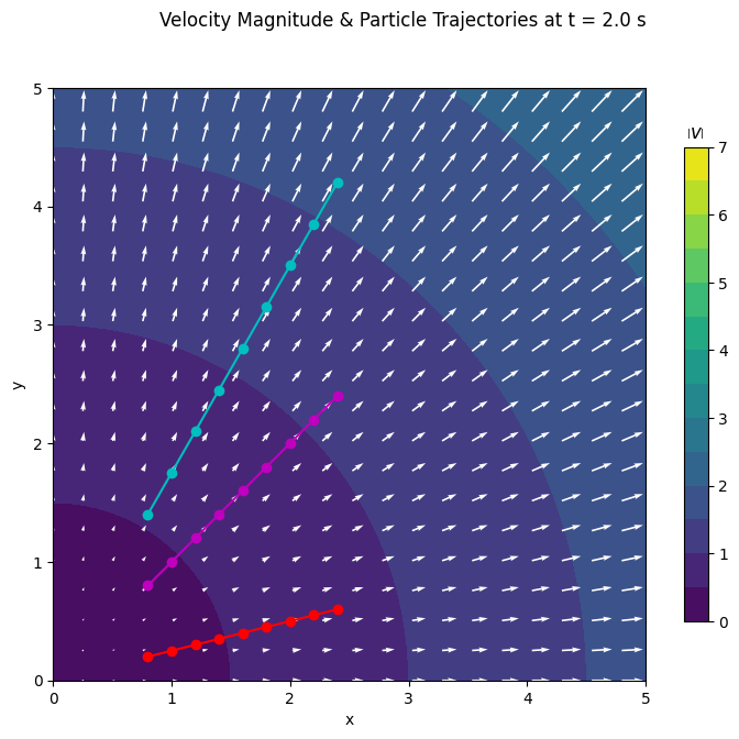
We see from this example that each particle moves the same distance in each time interval. In other words, each particle moves at a constant velocity and experiences no acceleration \(a_i = 0\).

Is this what we expect? In the lecture, we considered the material description of position \(\x'\), by noting that the spatial velocity field is equivalent to the partial derivative of a particle’s position with respect to time:

\[v_i=\frac{kx_i}{(1+kt)} = \frac{\partial x_i'}{\partial t} .\]

Thus, by integrating with respect to time we derive the material description of position:

\[x_i'(\mathbf{\xi}, t) = (1+kt)\xi_i = \xi_i + kt\xi_i \ ,\]

where \(\xi_i\) is the \(i^\textrm{th}\) component of the initial position of the material and \(kt\xi_i\) is the displacement of the particle as a function of time. As \(k\) is a constant, this shows that for a given initial position the particle does indeed move a constant distance in the same time (or at a constant velocity).

Exercise 1

Implement this equation for the material position as a function of time in the plot above and show that it gives the same results as our numerical integration (to some numerical precision).

def material_position(xi_x, xi_y, t, k=1):
    return (1+k*t)*xi_x, (1+k*t)*xi_y

# Define the particle position using our analytical function
for it in range(1, nt):
    px[:, it], py[:, it] = material_position(px[:, 0], py[:, 0], tt[it], k=k)

# Plot the velocity field at time zero
plt.figure(figsize=(9,7))
plt.subplot(aspect='equal')
plt.suptitle("Velocity Magnitude & Particle Trajectories at t = %1.1f s" % tt[-1])
plt.xlabel('x')
plt.ylabel('y')

# Define a sensible fixed colorscale
cc = np.arange(0, 7.5, 0.5)
cl = np.arange(0, 8, 1)

# Contour plot of velocity magnitude
c = plt.contourf(X, Y, vmag, cc)
cbar = plt.colorbar(c, shrink=0.8, ticks=cl)
cbar.ax.set_title("$\\left| v \\right|$")

# Quiver plot of velocity vector field
plt.quiver(X[::5,::5], Y[::5,::5], vx[::5,::5], vy[::5,::5], color='w')

# Marker plots of tracer particles, plot every 5th timestep
plt.plot(px[0,::5], py[0,::5], 'ro-')
plt.plot(px[1,::5], py[1,::5], 'mo-')
plt.plot(px[2,::5], py[2,::5], 'co-')

plt.show()

Relating spatial and material descriptions

Note that the expression above tells us the position \(x_i'\) of a particle at time that was at the original position \(\vector{\xi}\). If this expression is invertible (as it is in this case), we can rearrange it to give the initial position of a particle that is at any position \(\x\) in the flow at time \(t\):

\[\xi(\x, t) = \frac{x_i}{(1+kt)}\ .\]

This allows us to convert between the spatial and material description of position.

Exercise 2

Let’s consider a similar problem, but defined the other way round. Suppose that we know the material description of position, such that the motion of a particle of the continuum is described as:

\[x' = \xi_1 + kt\xi_2 \ , \, y' = \xi_2 + kt\xi_2 \ .\]

Note that in this case the displacement of the particle in \(x\) and \(y\) depends only on \(\xi_2\) (the original \(y\) position).

(a) Obtain the velocity of a particle in the material \(\mathbf{v}(\mathbf{\xi}, t)\) and spatial \(\v(\x, t)\) description.

(b) Modify the functions above for the new spatial velocity field and material position and visualise the pathlines.

(c) Sketch how a unit square with one corner at the origin is deformed by the field after one second and two seconds.

Exercise 3 (Optional)

If you are confused by the examples above and want to consider a simpler scenario to better understand these concepts, try to repeat this exercise with a simpler velocity field.

For example, consider the spatial description of a velocity field:

\[ v_i = k \ .\]

In other words, the velocity field is constant everywhere; it does not depend on time or position.

(a) Integrate this expression with respect to time to derive the material description of position with time.

(b) Plot the velocity field and pathlines of particles in this case.

Exercise 4 (Advanced)

• Try a velocity field that does not lead to a zero acceleration.

• Change initial tracer positions to get a further idea of how tracers move in different parts of the velocity field

Time derivative

The time derivative of any quantity in the material description is given by:

\[\frac{DP}{Dt} = \frac{\partial P}{\partial t} + \v \cdot \nabla P,\]

where:

• \(P\) is the quantity of interest, which could be a scalar, vector or tensor field;

• \(\v\) is the spatial description of the velocity vector field;

• \(\nabla P\) is the gradient of \(P\).

In the lecture, we used this expression to derive the material description of acceleration (the rate of change of velocity with time) for our example velocity field. We found that the acceleration in the material description was zero, implying that any particle in the flow experiences no acceleration, exactly as shown above.

Exercise 5

Consider the temperature field in spatial coordinates \(\x\) described by:

\[T(\x, t) = \alpha(x + y)\]

(a) Find the material description of temperature if a particle is moving through the temperature field according to:

\[x' = \xi_1 + kt\xi_2 \ , \, y' = \xi_2 + kt\xi_2 \ ,\]

where \(k\) is a constant as before.

(b) Determine the material time derivative of the temperature in both material and spatial descriptions.

Exercise 6 (Optional)

(a) For the same temperature field, find the material description of temperature if the spatial velocity field is given by:

\[v_i=\frac{kx_i}{(1+kt)},\]

where \(k\) is a constant.

(b) Determine the material time derivative of the temperature in both material and spatial descriptions.

(c) Modify the plotting code above to show the temperature field (rather than velocity magnitude), underneath the velocity vector field and pathlines.

Infinitesimal strain

Strain and rotation tensors

In the lecture we derived the infinitesimal strain tensor \(\tensor{\epsilon}\), which describes internal deformation of material in a displacement field. It is related to the displacement gradient by:

\[\tensor{\epsilon} = \frac{1}{2}\left(\nabla \u + \nabla\u^T\right) ,\]

where the displacement gradient is defined in Cartesian coordinates as:

\[\begin{split}\nabla \u = \frac{\partial u_j}{\partial x_i} = \left[\begin{array}{ccc} \frac{\partial u_1}{\partial x_1} & \frac{\partial u_2}{\partial x_1} & \frac{\partial u_3}{\partial x_1} \\ \frac{\partial u_1}{\partial x_2} & \frac{\partial u_2}{\partial x_2} & \frac{\partial u_3}{\partial x_2} \\ \frac{\partial u_1}{\partial x_3} & \frac{\partial u_2}{\partial x_3} & \frac{\partial u_3}{\partial x_3} \end{array} \right] .\end{split}\]

Note also that the rotation tensor \(\tensor{\omega}\) is defined as:

\[\tensor{\omega} = \frac{1}{2}\left(\nabla \u - \nabla\u^T\right) .\]

The transpose displacement gradient tensor is the sum of strain and rotation tensors.

\[ \nabla \u = \tensor{\epsilon} + \tensor{\omega}.\]

Strain tensor components

Similar to the stress tensor, we can define the following results:

• \(\tensor{\epsilon} \cdot \ex = \vector{d\ex}' = (\epsilon_{11}, \epsilon_{21}, \epsilon_{31})\) is the change in the unit vector in the \(x_1\) direction caused by the deformation.

• \(\ex \cdot \tensor{\epsilon} \cdot \ex = \epsilon_{11}\) is the unit elongation in the \(x_1\) direction. In other words, it is the change in length in the \(x_1\) direction of \(\ex\).

• \(\ex \cdot \tensor{\epsilon} \cdot \ey = \epsilon_{12}\) is the change of the \(\ey\) unit vector in the \(x_1\) direction. Because the strain tensor is symmetric, this is the same as the change of the \(\ex\) unit vector in the \(x_2\) direction \(\epsilon_{21}\). Note also that so long as the change is small, \(2\epsilon_{12}\) is the change in the angle of a unit square, spanned by \(\ex\) and \(\ey\).

More generally,

• \(\tensor{\epsilon}\cdot \hat{\x} = \vector{dx}'\), where the deformation of \(\hat{\x}\) by strain \(\tensor{\epsilon}\) results in the new vector \(\x' = \hat{\x} + \vector{dx}'\);

• \(\hat{\x} \cdot \tensor{\epsilon}\cdot \hat{\x} = \hat{\x} \cdot \vector{dx}'\), which is the component of the deformation \(\vector{dx}'\) in the direction of \(\hat{\x}\).

Exercise 7

With reference to a rectangular Cartesian coordinate system, the state of strain at a point is given by:

\[\begin{split} \tensor{\epsilon} = \left[\begin{array}{rrr} 5 & 3 & 0 \\ 3 & 4 & -1 \\ 0 & -1 & 2 \end{array} \right] \times 10^{-4} \ .\end{split}\]

(a) What is the unit elongation (change in length divided by original length) in the direction of \(2\ex + 2\ey + \ez\)?

(b) What is the change in angle between two vectors emanating from a point in the directions \(2\ex + 2\ey + \ez\) and \(3\ex - 6\ez\), which are perperpendicular prior to deformation?

Displacement and strain fields

In the lecture, we considered an example displacement field to develop our insight into strain.

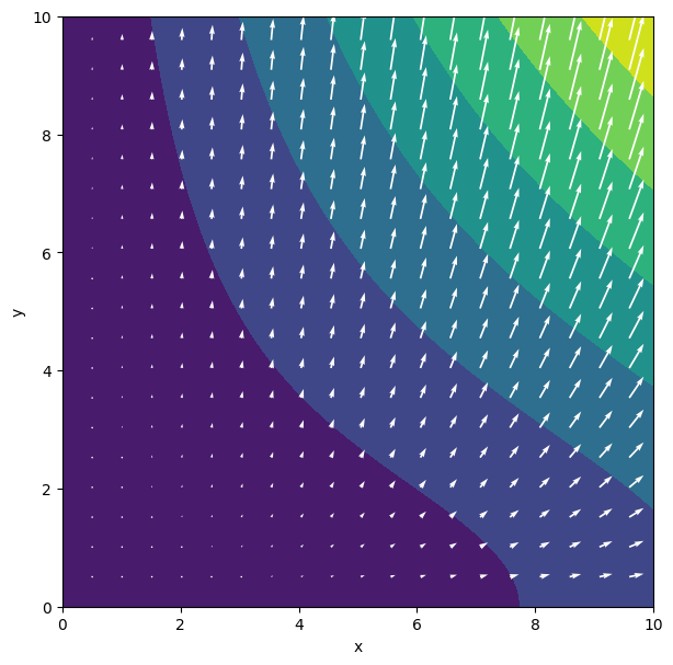
We considered the displacement field: \(u_x = 0.1x^2, \, u_y = 0.4xy\). Let’s have a look at this field.

# Let's define our displacement field. . .
def displacement_spatial(x, y, k1=0.1, k2=0.4):
    return k1*x**2, k2*x*y

# Visualise the displacement field 
# Define a grid, displacement vector field and displacement magnitude scalar field
k1=0.1; k2=0.4
X, Y = init_grid()
ux, uy = displacement_spatial(X, Y, k1=k1, k2=k2)
umag = np.sqrt(ux**2 + uy**2)

# Plot the fields
plt.figure(figsize=(9,7))
plt.subplot(aspect='equal')
plt.contourf(X, Y, umag)
plt.quiver(X[5::5,5::5], Y[5::5,5::5], ux[5::5,5::5], uy[5::5,5::5], color='w')
plt.xlabel('x')
plt.ylabel('y')

Text(0, 0.5, 'y')

We see that the field is quite complex. Can you anticipate what type of deformation such a field would result in? This is what the strain tensor tells us, so let’s remind ourselves of how we determine this.

For this field the displacement gradient tensor \(\nabla \u\) is:

\[\begin{split}\nabla \u = \left[\begin{array}{cc} \frac{\partial u_x}{\partial x} & \frac{\partial u_y}{\partial x} \\ \frac{\partial u_x}{\partial y} & \frac{\partial u_y}{\partial y} \end{array} \right] ,\end{split}\]

Which is:

\[\begin{split}\nabla \u = \left[\begin{array}{cc} 0.2 x & 0.4 y \\ 0 & 0.4x \end{array} \right] ~~~~or~~~~ \nabla^T \u = \left[\begin{array}{cc} 0.2 x & 0 \\ 0.4y & 0.4x \end{array} \right].\end{split}\]

Let’s visualise the displacement gradients for our field using a scalar field to represent each component of the \(\nabla \u\).

# Define the gradient of the displacement field for our example,
# which we have derived by hand.
# You can modify this function for different displacement fields. . .
def gradient_displacement(x, y, k1=0.1, k2=0.4):
    duxdx = 2*k1*x
    duydx = k2*y
    duxdy = 0*x
    duydy = k2*x
    return duxdx, duydx, duxdy, duydy

# Calculate the displacement gradient component fields
duxdx, duydx, duxdy, duydy = gradient_displacement(X, Y, k1=k1, k2=k2)

# Plot the transpose displacement gradient 
# as four separate scalar fields with the same colorscale
plot_2D_tensor_field(X, Y, duxdx, duydx, duxdy, duydy, cmax=4.)

<Figure size 640x480 with 0 Axes>

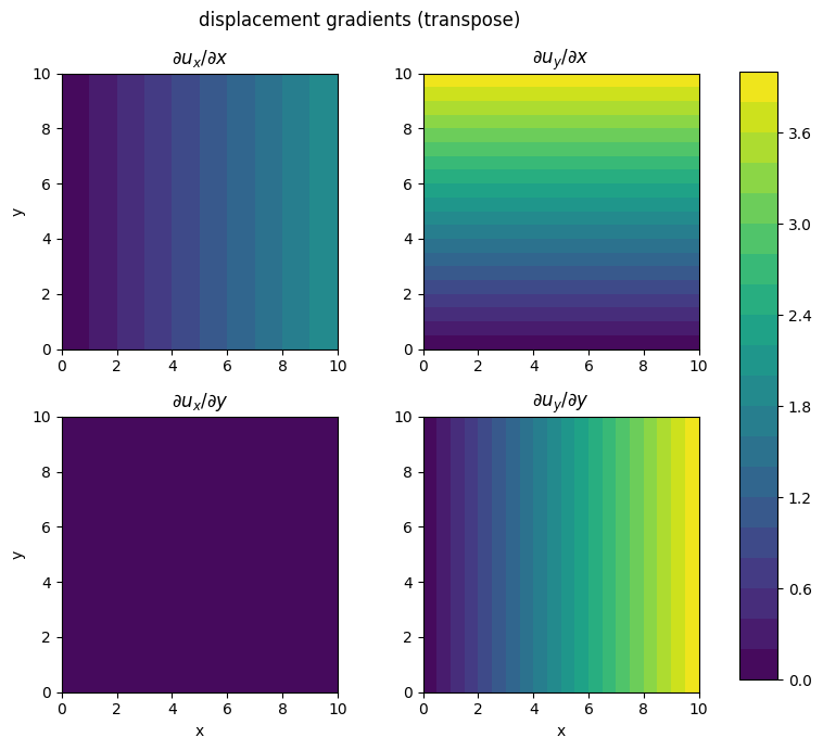
From this we see that the elongation in the \(x\) and \(y\) directions increases in the \(x\)-direction. There is no simple shear in the \(x\)-direction–i.e., initially vertical lines will remain vertical. The simple shear in the \(y\)-direction increases with \(y\).

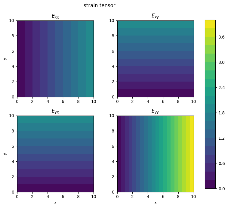
Armed with the displacement gradients, we can now calculate the infinitesimal strain tensor field:

\[\tensor{\epsilon} = \frac{1}{2}\left(\nabla \u + \nabla\u^T\right) .\]

Let’s visualise this in a similar way with a scalar field for each component of the tensor…

# Define a function for calculating the 2D strain tensor components 
# from the displacement gradients. . .
def strain_tensor_2D(x, y, k1, k2):
    
    # Calculate the displacement gradients
    duxdx, duydx, duxdy, duydy = gradient_displacement(X, Y, k1=k1, k2=k2)

    # Construct the strain tensor
    Exx = duxdx
    Exy = 0.5*(duxdy + duydx)
    Eyx = Exy
    Eyy = duydy
    
    return Exx, Exy, Eyx, Eyy

# Calculate the strain tensor component fields
Exx, Exy, Eyx, Eyy = strain_tensor_2D(X, Y, k1, k2)

# Plot the displacement gradient as four separate scalar fields with the same colorscale
plot_2D_tensor_field(X, Y, Exx, Exy, Eyx, Eyy, cmax=4., field='strain')

<Figure size 640x480 with 0 Axes>

We can notice a few things:

• The diagonal components are both positive everywhere, implying that shapes will increase in area when deformed.

• Elongation in the \(y\)-direction is greater than in the \(x\)-direction (\(\epsilon_{yy} > \epsilon_{xx}\)).

• Elongation in both directions increases with \(x\), but is constant in \(y\).

• The strain tensor is symmetric, so the shear strains \(\epsilon_{xy}\) and \(\epsilon_{yx}\) are the same.

With this insight, let’s now look at how some simple shapes (squares) are deformed by the displacement field.

def move_tracers(px, py, nt, dt=0.02, k1=0.1, k2=0.4):
    for i in range(1,nt):
        uxp, uyp = displacement_spatial(px[:,i-1], py[:,i-1], k1=k1, k2=k2)
        px[:,i] = px[:,i-1] + uxp * dt
        py[:,i] = py[:,i-1] + uyp * dt
    return px, py

nt=81
# Define two squares formed by five tracers (with one overlap for plotting) 
px1, py1 = tracers(p0=[[0.6, 1.6], [1.2, 1.6], [1.2, 2.2], [0.6, 2.2], [0.6, 1.6]], nt=nt)
px2, py2 = tracers(p0=[[1.6, 0.6], [1.6, 1.2], [2.2, 1.2], [2.2, 0.6], [1.6, 0.6]], nt=nt)

# Move the tracers in the displacement field for nt increments
px1, py1 = move_tracers(px1, py1, 81)
px2, py2 = move_tracers(px2, py2, 81)

# Plot the fields
plt.set_cmap("viridis")
plt.figure(figsize=(9,7))
plt.subplot(aspect='equal')
plt.contourf(X, Y, umag)
plt.quiver(X[5::5,5::5], Y[5::5,5::5], ux[5::5,5::5], uy[5::5,5::5], 
           color='w', scale=50, scale_units='inches')
plt.plot(px1[:,0], py1[:,0], 'wo-')
plt.plot(px1[:,-1], py1[:,-1], 'ro-')
plt.plot(px2[:,0], py2[:,0], 'wo-')
plt.plot(px2[:,-1], py2[:,-1], 'ro-')
plt.xlabel('x')
plt.ylabel('y')
plt.show()

<Figure size 640x480 with 0 Axes>

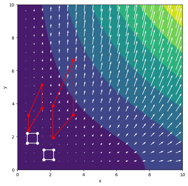
Here we see that the square on the right has undergone more extension in \(x\) and \(y\) (as well as more translation), but has been sheared slightly less in the \(y\) direction. The sides of the square that were vertical have not been rotated, while the initially horizontal sides have been rotated.

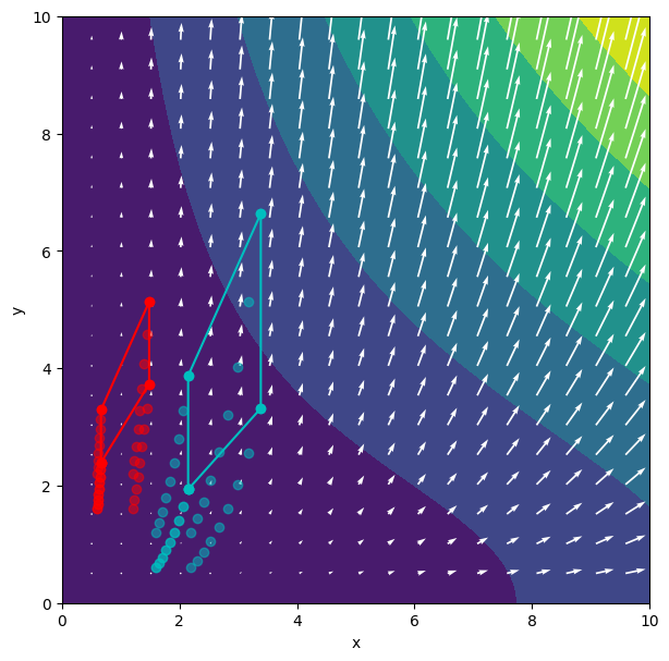
We can also plot the pathlines of the corner points to visualise the stages of deformation.

# Plot the tracer positions vs time. . .
plt.set_cmap("viridis")
plt.figure(figsize=(9,7))
plt.subplot(aspect='equal')
plt.contourf(X, Y, umag)
plt.quiver(X[5::5,5::5], Y[5::5,5::5], ux[5::5,5::5], uy[5::5,5::5], 
           color='w', scale=50, scale_units='inches')
plt.plot(px1[:,::10], py1[:,::10], 'ro', alpha=0.5)
plt.plot(px1[:,-1], py1[:,-1], 'ro-')
plt.plot(px2[:,::10], py2[:,::10], 'co', alpha=0.5)
plt.plot(px2[:,-1], py2[:,-1], 'co-')
plt.xlabel('x')
plt.ylabel('y')
plt.show()

<Figure size 640x480 with 0 Axes>

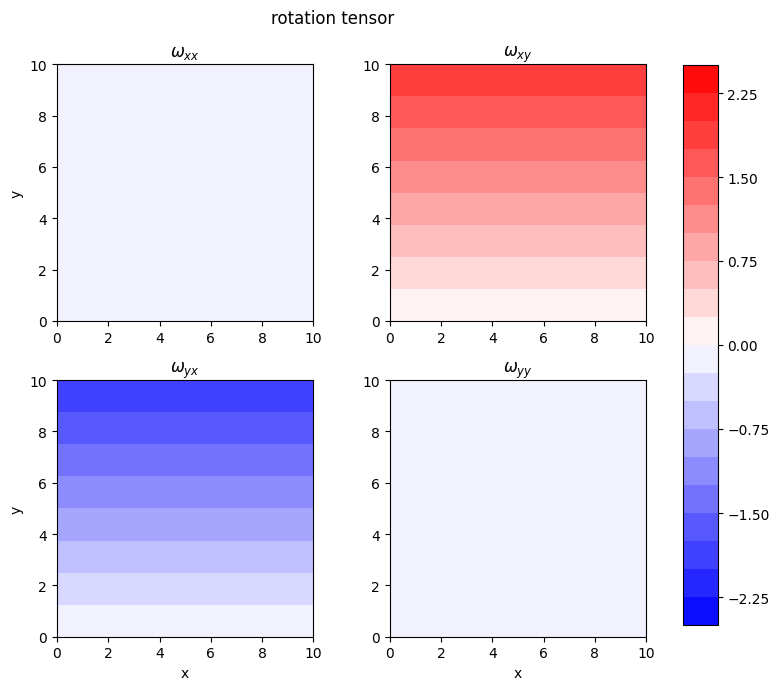
We can also visualise the rotation tensor in a similar way.

Recall that the rotation tensor in 2D Cartesian coordinates is given by:

\[\tensor{\omega} = \frac{1}{2}\left(\nabla \u - \nabla\u^T\right) .\]

# Define a function for calculating the 2D rotation tensor components 
# from the displacement gradients. . .
def rotation_tensor_2D(x, y, k1, k2):
    
    # Calculate the displacement gradients
    duxdx, duydx, duxdy, duydy = gradient_displacement(X, Y, k1=k1, k2=k2)

    # Construct the strain tensor
    Wxx = 0.*x
    Wxy = 0.5*(duydx - duxdy)
    Wyx = 0.5*(duxdy - duydx)
    Wyy = 0.*x
    
    return Wxx, Wxy, Wyx, Wyy

# Calculate the strain tensor component fields
Wxx, Wxy, Wyx, Wyy = rotation_tensor_2D(X, Y, k1, k2)

# Plot the displacement gradient as four separate scalar fields with the same colorscale
plot_2D_tensor_field(X, Y, Wxx, Wxy, Wyx, Wyy, cmin=-2.5, cmax=2.5, field='rotation')

<Figure size 640x480 with 0 Axes>

Exercise 8 (Optional)

If you find the example above too complicated and/or you would like to develop more intuition about the deformation described by different displacement fields and strain tensors, you might like to implement different displacement_spatial functions and their corresponding gradient_displacement function, which you will have to work out by hand.

Some displacement fields you might analyse, in order of complexity are:

Pure translation: $\(u_x = k_1, \, u_y = k_2\)$

Pure rotation: $\(u_x = k_1y, \, u_y = -k_2x\)$

Pure shear: $\(u_x = k_1x, \, u_y = -k_2y\)$

Principal strains and strain invariants

As with the stress tensor, we can define a rotated coordinate system in which the strain tensor is diagonal–i.e., all off-diagonal components are zero. The diagonal components of this tensor are the principal strains (maximum, minimum and intermediate fractional length changes) and the corresponding coordinate directions are the principal strain directions.

To find the principal strains and associated directions we need to solve the eigenvalue problem for the strain tensor.

We can also define measures of strain that are invariant to the coordinate system. For example, the trace of the strain tensor (the sum of the diagonal components) is the volume change associated with the deformation.

\[ \mathrm{tr}(\tensor{\epsilon}) = \theta = \epsilon_{ii} .\]

Finally, we can separate the total strain tensor into an isotropic and deviatoric part:

\[\epsilon_{ij} = \frac{\theta}{3}\delta_{ij} + \epsilon_{ij}' .\]

where \(\epsilon_{ij}'\) is known as the deviatoric strain. The isotropic part describes volume change only; the deviatoric part describes change in shape only and involves no change in volume.

Exercise 9

For the displacement field \(u_1 = k\xi_1^2, \, u_2 = k\xi_2\xi_3, \, u_3 = k(2\xi_1\xi_3 + \xi_1^2)\) and \(k = 10^{-6}\), find:

(a) the infinitesimal strain tensor \(\tensor{\epsilon}\)

(Advanced)

(b) the maximum unit elongation for an element initially at \(\xi = (1, 0, 0)\).

Strain rate

In similar way as for the strain tensor, a tensor that describes the rate of change of deformation can be defined from the velocity gradient:

\[\begin{split}\nabla \v = \frac{\partial v_i}{\partial x_j} = \left[\begin{array}{ccc} \frac{\partial v_1}{\partial x_1} & \frac{\partial v_2}{\partial x_1} & \frac{\partial v_3}{\partial x_1} \\ \frac{\partial v_1}{\partial x_2} & \frac{\partial v_2}{\partial x_2} & \frac{\partial v_3}{\partial x_2} \\ \frac{\partial v_1}{\partial x_3} & \frac{\partial v_2}{\partial x_3} & \frac{\partial v_3}{\partial x_3} \end{array} \right] .\end{split}\]

The strain rate tensor \(\tensor{D}\) is defined as:

\[\tensor{D} = \frac{1}{2}\left(\nabla \v + \nabla\v^T\right) .\]

The vorticity tensor \(\tensor{W}\) is defined as:

\[\tensor{W} = \frac{1}{2}\left(\nabla \v - \nabla\v^T\right) .\]

The velocity gradient tensor is the sum of strain rate and vorticity tensors.

\[ \nabla \v = \tensor{D} + \tensor{W}.\]

Finite strain

The infinitesimal strain tensor and our analysis up to this point has assumed that in any given increment of deformation, the strain is small or, equivalently, that the displacement gradient is constant over the strain increment. For non-linear displacement fields, this assumption will not be valid and so we must either apply the infinitesimal strain tensor many times in small increments to describe the deformation or use so-called finite strain theory, which uses fewer approximations to describe deformation.

Recall that the deformation of an element \(\vector{dx}'\) caused by a displacement field is given by:

\[\vector{dx}' = \vector{dx} + \nabla{\u}\cdot\vector{dx} .\]

It can be shown that according to finite strain theory, the finite deformation tensor (or Lagrange strain tensor) \(\tensor{E^*}\) is defined as:

\[\tensor{E^*} = \frac{1}{2}\left[\nabla\u + (\nabla\u)^T + (\nabla\u)^T\cdot\nabla\u\right] ,\]

which we note includes extra terms \((\nabla\u)^T.\nabla\u\) that are not part of the infinitesismal strain tensor \(\tensor{E}\). As a result, the components of \(\tensor{E^*}\) and \(\tensor{\epsilon}\) will differ for large strains and have slightly different interpretations. The advanced exercise below will help build your intuition for this.

Exercise 10 (Advanced)

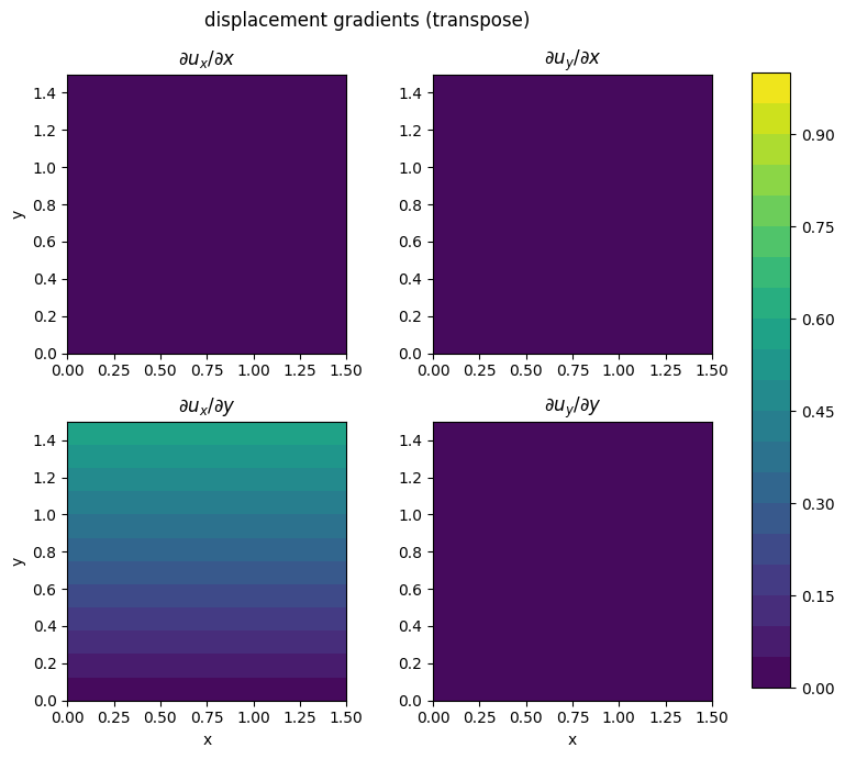
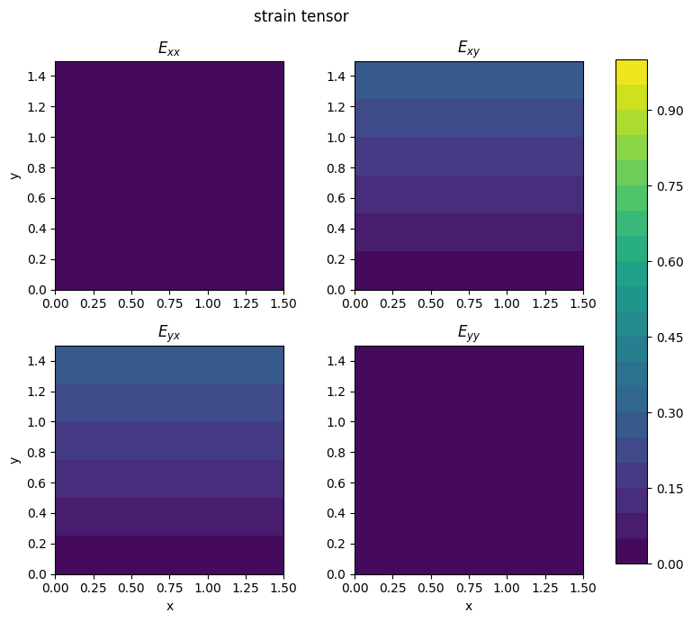
Given the 2D displacement field: \(u_1= k\xi_2^2\), \(u_2=0\), where \(k=10^{-4}\):

(a) Sketch the deformation of a unit square OABC, with as corner points: \(O=(0,0)\), \(A=(1,0)\), \(B=(1,1)\), \(C(0,1)\).

(b) Calculate \(\nabla\u\), \((\nabla\u)^T\) and \((\nabla\u)^T.\nabla\u\) and therefore write down the Lagrange strain tensor \(\tensor{E^*}\).

(c) Using the displacement gradient \(\nabla\u\) directly (i.e., not by calculating the infinitesimal strain tensor), find the deformed vectors \(\vector{dx}'^{(1)}\) and \(\vector{dx}'^{(2)}\) of the material elements \(\vector{d\xi}^{(1)} = d\xi_1\ex\) and \(\vector{d\xi}^{(2)} = d\xi_2\ey\), which were originally at point C(0,1).

(d) Determine the difference between the deformed and undeformed lengths of the two elements.

(e) Determine the change in angle between the two elements.

(f) Obtain the infinitesimal strain tensor \(\tensor{\epsilon}\).

(g) Estimate the unit elongation for material elements \(\vector{d\xi}^{(1)} = d\xi_1\ex\) and \(\vector{d\xi}^{(2)} = d\xi_2\ey\) using the infinitesimal strain tensor \(\tensor{\epsilon}\).

(h) And also find the decrease in angle between these two elements from the strain tensor \(\tensor{\epsilon}\).

(i) Compare the answers from (g), (h) and (d), (e).

# Let's define our displacement field. . .
def displacement_spatial(x, y, k1=0.4, k2=0.4):
    #Return a field of k1, k2 rather than scalars. . .
    return k1*y**2, 0*y 

# Gradients are all zero everywhere
def gradient_displacement(x, y, k1=0.4, k2=0.4):
    duxdx = 0*x
    duydx = 0*y
    duxdy = 2*k1*y
    duydy = 0*x
    return duxdx, duydx, duxdy, duydy

# Let's visualise this strain field. If we use k=1.E-4, we won't see any deformation,
# so let's set this as 0.2 to exaggerate the effects of the deformation. . .
k1=0.2; k2=0

# Define the constants of the displacement field and number of strain increments
nt=81

# Define one squares formed by five tracers (with one overlap for plotting) 
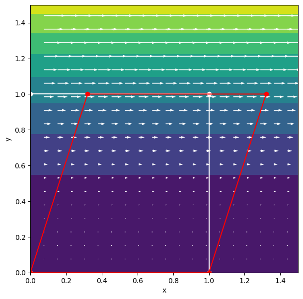
px1, py1 = tracers(p0=[[0., 0.], [1., 0.], [1., 1.], [0., 1.], [0., 0.]], nt=nt)

# Define the displacement field and magnitude
X, Y = init_grid(Lx=1.5, Ly=1.5)
ux, uy = displacement_spatial(X, Y, k1=k1, k2=k2)
umag = np.sqrt(ux**2 + uy**2)

# Move the tracers in the displacement field for nt increments
px1, py1 = move_tracers(px1, py1, 81, k1=k1, k2=k2)

# Calculate the displacement gradient component fields
duxdx, duydx, duxdy, duydy = gradient_displacement(X, Y, k1=k1, k2=k2)

# Plot the displacement gradient as four separate scalar fields with the same colorscale
plot_2D_tensor_field(X, Y, duxdx, duydx, duxdy, duydy, cmax=1.)

# Calculate the strain tensor component fields
Exx, Exy, Eyx, Eyy = strain_tensor_2D(X, Y, k1, k2)

# Plot the displacement gradient as four separate scalar fields with the same colorscale
plot_2D_tensor_field(X, Y, Exx, Exy, Eyx, Eyy, cmax=1., field='strain')

# Plot the fields
plt.set_cmap("viridis")
plt.figure(figsize=(9,7))
plt.subplot(aspect='equal')
plt.contourf(X, Y, umag)
plt.quiver(X[5::5,5::5], Y[5::5,5::5], ux[5::5,5::5], uy[5::5,5::5], color='w')
plt.plot(px1[:,0], py1[:,0], 'wo-')
plt.plot(px1[:,-1], py1[:,-1], 'ro-')
plt.xlabel('x')
plt.ylabel('y')

Text(0, 0.5, 'y')

<Figure size 640x480 with 0 Axes>