Exercises

Chapter 2: Stress and Tensors

Learning outcomes

At the end of this session you should be able to:

1. Interpret different components of 3D Cauchy stress tensor.

2. Decompose a rank 2 tensor into symmetric and anti-symmetric components

3. Determine state of stress on given plane

4. Transform rank 2 tensor to a new basis.

Table of Contents

• 1  Stress
• 1.1  Cauchy stress tensor
• 1.2  Traction
• 1.3  Normal and shear stress
• 1.3.1  Exercise 1
• 1.3.2  Exercise 2
• 2  Transforming stress to a new orthonormal basis
• 2.0.1  Exercise 3
• 3  Special stress components
• 3.1  Stress invariants
• 3.2  Extra: Principal stresses
• 3.2.1  Exercise 4
• 3.2.2  Exercise 5
• 3.3  Deviatoric stress and invariants
• 3.3.3  Exercise 6

Types of content

Exercises for all

Optional additional practise

Optional advanced practise/content

Settings for notebook

# Import packages for notebook here
import numpy as np
import matplotlib.pyplot as plt

%matplotlib inline

Do not alter this cell. LaTeX commands for frequently used terms.

\[\newcommand{\tensor}[1]{\underline{\underline{\mathbf{#1}}}}\]

\[\newcommand{\vector}[1]{\mathbf{#1}}\]

\[\newcommand{\matrix}[1]{\mathbf{#1}}\]

\[\newcommand{\det}[1]{\mathrm{det}\left(#1\right)}\]

\[\newcommand{\ex}{\vector{\hat{e}}_1}\]

\[\newcommand{\ey}{\vector{\hat{e}}_2}\]

\[\newcommand{\ez}{\vector{\hat{e}}_3}\]

\[\newcommand{\nhat}{\vector{\hat{n}}}\]

\[\newcommand{\ehat}{\vector{\hat{e}}}\]

\[\newcommand{\xhat}{\vector{\hat{x}}}\]

\[\newcommand{\x}{\vector{x}}\]

\[\newcommand{\v}{\vector{v}}\]

\[\newcommand{\u}{\vector{u}}\]

Stress

Cauchy stress tensor

Stress (force per unit area) in a body is the response to forces acting on the body. It is a (2nd-order) tensor quantity as it depends on direction in two ways: the direction of the force acting on a plane and the direction of the normal to the plane on which the force acts.

Stress is defined as positive if the force is in the same direction as the outward normal (tension); negative if it acts in the opposite direction (compression).

The stress tensor can be written as a square matrix \(\tensor{\sigma} = \sigma_{ij}\) and has algebraic properties similar to those of matrices.

In 3D the stress tensor has nine components; in 2D it has four.

\[\begin{split}\text{3D:} \, \tensor{\sigma} = \sigma_{ij} = \left[\begin{array}{ccc} \sigma_{11} & \sigma_{12} & \sigma_{13} \\ \sigma_{21} & \sigma_{22} & \sigma_{23} \\ \sigma_{31} & \sigma_{32} & \sigma_{33} \end{array} \right] , \ \ \ \ \text{2D:} \, \tensor{\sigma} = \sigma_{ij} = \left[\begin{array}{cc} \sigma_{11} & \sigma_{12} \\ \sigma_{21} & \sigma_{22} \end{array} \right] .\end{split}\]

The first index of the stress component is the orientation (outward normal direction) of the plane; the second is the orientation of the force.

The diagonal terms are normal stresses the off-diagonal terms are shear stresses.

Traction

If we are interested in the force (per unit area) acting at a point in the body on a given plane, the dot product of the transpose of the stress tensor with a unit vector \(\nhat\) gives the traction \(\vector{t}\) (effective force per unit area) acting on the plane normal to the unit vector.

\[\vector{t} = \tensor{\sigma}^T \cdot \nhat = \sigma_{ji} n_j. \]

For example, the traction in the \(x_1\) direction (\(\nhat = \ex = (1, 0, 0)^T\)) is given by:

\[\begin{split}\vector{t}_1 = \tensor{\sigma}^T \cdot \ex = \left[\begin{array}{ccc} \sigma_{11} & \sigma_{21} & \sigma_{31} \\ \sigma_{12} & \sigma_{22} & \sigma_{32} \\ \sigma_{13} & \sigma_{23} & \sigma_{33} \end{array} \right]\left[\begin{array}{r} 1 \\ 0 \\ 0 \end{array} \right] = \left[\begin{array}{r} \sigma_{11} \\ \sigma_{12} \\ \sigma_{13} \end{array} \right] .\end{split}\]

If we are interested in the component of this vector in a particular direction, we can do the dot product of another unit vector in the direction of interest \(\vector{\hat{p}}\) with the traction vector \(\vector{t}\).

\[\sigma_{pn} = \vector{\hat{p}} \cdot \vector{t} = \vector{\hat{p}} \cdot \tensor{\sigma}^T \cdot \nhat = p_i\sigma_{ji}n_j .\]

For example, going back to our traction in the \(x_1\) direction \(\vector{t}_1\), the component of this in the \(\ex\) direction is:

\[\begin{split}\ex \cdot \vector{t}_1 = \left[\begin{array}{ccc} 1 & 0 & 0 \\ \end{array} \right]\left[\begin{array}{r} \sigma_{11} \\ \sigma_{12} \\ \sigma_{13} \end{array} \right] = \sigma_{11} ,\end{split}\]

or

\[\begin{split}\ex \cdot \tensor{\sigma}^T \cdot \ex = \left[\begin{array}{ccc} 1 & 0 & 0 \\ \end{array} \right] \left[\begin{array}{ccc} \sigma_{11} & \sigma_{21} & \sigma_{31} \\ \sigma_{12} & \sigma_{22} & \sigma_{32} \\ \sigma_{13} & \sigma_{23} & \sigma_{33} \end{array} \right]\left[\begin{array}{r} 1 \\ 0 \\ 0 \end{array} \right] = \sigma_{11} .\end{split}\]

and the component in the \(\ey\) direction is:

\[\begin{split}\ey \cdot \vector{t}_1 = \left[\begin{array}{ccc} 0 & 1 & 0 \\ \end{array} \right]\left[\begin{array}{r} \sigma_{11} \\ \sigma_{12} \\ \sigma_{13} \end{array} \right] = \sigma_{12} ,\end{split}\]

or

\[\begin{split}\ey \cdot \tensor{\sigma}^T \cdot \ex = \left[\begin{array}{ccc} 0 & 1 & 0 \\ \end{array} \right] \left[\begin{array}{ccc} \sigma_{11} & \sigma_{21} & \sigma_{31} \\ \sigma_{12} & \sigma_{22} & \sigma_{32} \\ \sigma_{13} & \sigma_{23} & \sigma_{33} \end{array} \right]\left[\begin{array}{r} 1 \\ 0 \\ 0 \end{array} \right] = \sigma_{12} .\end{split}\]

Normal and shear stress

We can also think of the traction vector \(\vector{t}\) as comprising a normal component \(\vector{t}_n\) and a shear component \(\vector{t}_s\). In 3D, the total shear component will be the vector sum of the two shear components orthogonal to the normal component.

Exercise 1

Given a stress tensor (units MPa) at a point in a body:

\[\begin{split}\tensor{\sigma} = \left[\begin{array}{rrr} 1 & 2 & 3 \\ 2 & 4 & 5 \\ 3 & 5 & 0 \end{array} \right] .\end{split}\]

(a) Find the normal stresses on the coordinate planes through the point with normal in \(\ex\) and \(\ez\) direction.

(b) Find the total shear stresses on the two planes from (a).

(c) Find the traction on a plane through the point with normal in the direction of \(2\ex + 2\ey + \ez\).

Exercise 2

Consider that at a point in a continuum the stress state is such that \(\sigma_{11} =1\) MPa and \(\sigma_{22} =-1\) MPa and all other stress components \(\sigma_{ij}=0\).

(a) Show that the only plane on which the stress vector is zero, is the plane with normal in the \(\ez\) direction.

(b) Give three planes on which no normal stress is acting.

Transforming stress to a new orthonormal basis

In the lecture we showed that by resolving forces acting on an aribtrary plane and maintaining the force balance, we can define the normal and shear stress on the plane.

For a 2D stress state, we saw that for a plane with an outward normal oriented at an angle of \(\phi\) clockwise (\(-\phi\) anti-clockwise) from the \(x_2\) axis, the normal \(\sigma_{nn}\) and shear stress \(\sigma_{ns}\) components are given by:

\[\sigma_{nn} = \sigma_{11} \sin^2\phi + \sigma_{12} \sin\phi\cos\phi + \sigma_{21} \sin\phi\cos\phi + \sigma_{22} \cos^2\phi \]

and

\[\sigma_{ns} = \sigma_{11} \sin\phi\cos\phi - \sigma_{12}\sin^2\phi + \sigma_{21} \cos^2\phi - \sigma_{22} \sin\phi\cos\phi .\]

We could also have found this result by: (1) calculating the traction vector on the plane with normal \(\nhat\) in the direction \(\phi\) degrees clockwise from the \(x_2\) axis: \(\nhat = (\sin\phi, \cos\phi)\):

\[\begin{split}\vector{t}_n = \tensor{\sigma}^T \cdot \nhat = \left[\begin{array}{cc} \sigma_{11} & \sigma_{21} \\ \sigma_{12} & \sigma_{22} \end{array} \right]\left[\begin{array}{c} \sin\phi \\ \cos\phi \end{array} \right] = \left[\begin{array}{c} \sigma_{11}\sin\phi + \sigma_{21}\cos\phi \\ \sigma_{12}\sin\phi + \sigma_{22}\cos\phi \end{array} \right] .\end{split}\]

Then (2) resolving the traction in the directions normal to the surface normal:

\[\begin{split}\sigma_{nn} = \nhat \cdot \vector{t}_n = \left[\begin{array}{cc} \sin\phi & \cos\phi \end{array} \right]\left[\begin{array}{c} \sigma_{11}\sin\phi + \sigma_{21}\cos\phi \\ \sigma_{12}\sin\phi + \sigma_{22}\cos\phi \end{array} \right],\end{split}\]

and parallel to the surface normal \(\vector{\hat{s}} = (\cos\phi, -\sin\phi)\):

\[\begin{split}\sigma_{ns} = \vector{\hat{s}} \cdot \vector{t}_n = \left[\begin{array}{cc} \cos\phi & -\sin\phi \end{array} \right]\left[\begin{array}{c} \sigma_{11}\sin\phi + \sigma_{21}\cos\phi \\ \sigma_{12}\sin\phi + \sigma_{22}\cos\phi \end{array} \right]. \end{split}\]

Importantly, this is equivalent to the tensor transformation that describes solid body rotation to a new orthonomal basis \(\{\ex', \ey'\}\):

\[ \tensor{\sigma}'^T = \matrix{A}\cdot\tensor{\sigma}^T\cdot\matrix{A}^T \]

where the columns of \(\matrix{A}^T\) are formed by the new basis vectors \(\{\ex', \ey'\}\):

\[\begin{split} \matrix{A}^T = \left[\begin{array}{cc} e_1e_1' & e_1e_2' \\ e_2e_1' & e_2e_2' \end{array} \right] = \left[\begin{array}{cc} \cos\phi & \sin\phi \\ -\sin\phi & \cos\phi \end{array} \right] .\end{split}\]

Or, if the components of \(\matrix{A}\) are written as \(\alpha_{ij}\), then \(\alpha_{ij} = \ehat_i'\cdot\ehat_j\).

Thus, we have:

\[\begin{split}\left[\begin{array}{cc} \sigma_{ss} & \sigma_{ns} \\ \sigma_{sn} & \sigma_{nn} \end{array} \right] = \left[\begin{array}{cc} \cos\phi & -\sin\phi \\ \sin\phi & \cos\phi \end{array} \right] \left[\begin{array}{cc} \sigma_{11} & \sigma_{21} \\ \sigma_{12} & \sigma_{22} \end{array} \right] \left[\begin{array}{cc} \cos\phi & \sin\phi \\ -\sin\phi & \cos\phi \end{array} \right] .\end{split}\]

Exercise 3

For the following state of stress (in MPa):

\[\begin{split}\tensor{\sigma} = \left[\begin{array}{rrr} 0 & 1 & 0 \\ 1 & 2 & 0 \\ 0 & 0 & 1 \end{array} \right] ,\end{split}\]

in a rectangular Cartesian coordinate system \(\left\{ \ex, \ey, \ez \right\}\), find \(\sigma_{11}'\), \(\sigma_{21}'\) and \(\sigma_{33}'\) on a new basis \(\left\{\ex', \ey', \ez'\right\}\) obtained by rotating about the \(\ez\) axis by 90\(^\circ\), such that \(\ex'=\ey\).

Special stress components

Stress invariants

Recall that stress is a tensor quantity and as such is the same regardless of coordinate system.

The matrix formed of the tensor components, however, will depend on the coordinate frame.

There are important measures of the stress tensor that are independent of the coordinate frame. These are called invariants, which can be expressed in different ways. Here are example definitions (more are given in the lecture notes):

\[I_1 = \text{tr}(\tensor{\sigma}) = \sigma_{ii}\]

\[I_2 = \text{minor}(\tensor{\sigma}) = \sigma_{11}\sigma_{22} + \sigma_{22}\sigma_{33} + \sigma_{11}\sigma_{33} - \sigma^2_{12} - \sigma^2_{23} - \sigma^2_{31} \]

\[I_3 = \det{\tensor{\sigma}}\]

Extra: Principal stresses

As the stress tensor is a real-valued, symmetric second-order tensor (i.e., square, symmetric matrix), it can be diagonalized.

This means a coordinate frame can be found, such that only the diagonal elements (normal stresses) remain.

For the stress tensor, these elements, \(\sigma_1\), \(\sigma_2\), \(\sigma_3\) are called the principal stresses.

Finding the principal stresses, and the corresponding principal directions (vectors), is equivalent to solving the eigenvalue problem for the stress tensor.

We seek \(\lambda\) that satisfies:

\[ \det{\tensor{\sigma}-\lambda\matrix{I}} = 0\]

to find the eigenvalues and then to find the eigenvectors \(\x\) we seek non-trivial solutions to:

\[ \left(\tensor{\sigma}-\lambda\matrix{I}\right)\cdot \x = \vector{0} .\]

As the stress tensor is symmetric, the eigenvectors will be orthogonal so the principal stress directions can form an orthonormal basis. If the principal stress directions are known, then finding the principal stresses can be cast as a change of orthonormal basis:

\[\begin{split} \left[\begin{array}{ccc} \sigma_{1} & 0 & 0 \\ 0 & \sigma_{2} & 0 \\ 0 & 0 & \sigma_{3} \end{array} \right] = \matrix{A} \cdot \tensor{\sigma} \cdot \matrix{A}^T , \end{split}\]

where the columns of linear transformation matrix \(\matrix{A}^T\) are the normalised principal stress directions \(\xhat_1\), \(\xhat_2\) and \(\xhat_3\).

When cast in this way, it should be apparent that the largest normal stress acting at a point is the largest (most negative) principal stress and the smallest (most positive) normal stress is the smallest principal stress.

Aside: In 2D, we can confirm this by considering the normal stress on a plane with a normal at an angle \(\phi\) clockwise from the second principal direction:

\[\sigma_{nn} = \sigma_{1} \sin^2\phi + \sigma_{2} \cos^2\phi .\]

which can be rewritten as:

\[\sigma_{nn} = \frac{\sigma_{1} + \sigma_{2}}{2} ( \sin^2\phi + \cos^2\phi ) + \frac{\sigma_{1} - \sigma_{2}}{2} ( \sin^2\phi - \cos^2\phi ).\]

\[\sigma_{nn} = \frac{\sigma_{1} + \sigma_{2}}{2} - \frac{\sigma_{1} - \sigma_{2}}{2} \cos2\phi.\]

From this we see that, for \(\sigma_1 > \sigma_2\), \(\sigma_{nn}\) is smallest (equal to \(\sigma_2\)) when \(\phi=0\), and largest (equal to \(\sigma_1\)) when \(\phi=90\) and in between for \(0 < \phi < 90\).

Note: If \(\sigma_1\) is largest and \(\sigma_3\) smallest principal stress, then the maximum shear stress is given by:

\[\left| \sigma_{s}^\text{max} \right|= \frac{\sigma_1-\sigma_3}{2}.\]

The maximum shear stress is important for modelling permanent deformation (plastic yielding).

Exercise 4

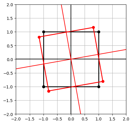
The code below shows how we can compute the components of the stress tensor in a rotated reference frame, given the tensor components in the standard basis and a rotation angle.

The code also plots the rotated coordinate system and confirms that the stress invariants are the same in the original and rotated frame.

Use this cell to investigate how the stress tensor components change as you rotate the coordinate frame. For the starting case:

\[\begin{split}\left[\begin{array}{cc} 2 & 1 \\ 1 & 3 \end{array} \right] ,\end{split}\]

what do you notice happens at approximately 58 degrees rotation?

# Print floats to only 2 d.p.
np.set_printoptions(precision=2, suppress=True)

# Define a stress tensor and print (remember that the stress tensor should be symmetric)
mS = np.array([[2., 1.],
              [1., 3.]])
assert np.allclose(mS,mS.T), "The stress tensor should be symmetric S = S^T"

print("\n The stress tensor in the standard coordinate basis:")
print(mS)

# Define a unit square for plotting rotation
mX = np.array([[-1,-1],
              [-1, 1],
              [ 1, 1],
              [ 1,-1],
              [-1,-1]]).T

# Define the rotation angle (positive anti-clockwise):
theta_deg = 10.
theta = np.deg2rad(theta_deg)
print("\n The rotation angle of the coordinate basis:")
print(theta_deg)

# Define the transformation matrices A and A^T (the latter has the new basis as columns)
mA = np.array([[np.cos(theta), np.sin(theta)],
              [-np.sin(theta), np.cos(theta)]])

# Deform the coordinate frame
mXp = mA.T @ mX

# Compute components of stress tensor in the rotated coordinate system
mSp = mA @ mS @ mA.T
print("\n The stress tensor in the rotated coordinate basis:")
print(mSp)

print("\n The basis vectors of the rotated coordinate system:")
print(mA.T)

# Stress invariants
print("\n The first and third invariants of the stress tensor (original and rotated):")
print("I_1 = %2.1f, %2.1f" % (np.trace(mS), np.trace(mSp)))
print("I_3 = %2.1f, %2.1f" % (np.linalg.det(mS), np.linalg.det(mSp)))

# The second invariant I_2 = minor(S) is left for you to code up. 
# You could write a function to do this in terms of the components of the matrix
# or the determinants of the minor matrices of S as given in the lecture notes. . . 

plt.subplot(aspect='equal')
plt.plot(mX[0,:], mX[1,:], 'ko-', lw=2)
plt.plot(mXp[0,:], mXp[1,:], 'ro-', lw=2)
plt.xlim(-2,2); plt.ylim(-2,2)
plt.axhline(0, color='k'); plt.axvline(0, color='k')
plt.plot([-3*mA.T[1,0],3*mA.T[1,0]],[3*mA.T[1,1],-3*mA.T[1,1]], 'r')
plt.plot([-3*mA.T[0,0],3*mA.T[0,0]],[-3*mA.T[1,0],3*mA.T[1,0]], 'r')
plt.grid()

 The stress tensor in the standard coordinate basis:
[[2. 1.]
 [1. 3.]]

 The rotation angle of the coordinate basis:
10.0

 The stress tensor in the rotated coordinate basis:
[[2.37 1.11]
 [1.11 2.63]]

 The basis vectors of the rotated coordinate system:
[[ 0.98 -0.17]
 [ 0.17  0.98]]

 The first and third invariants of the stress tensor (original and rotated):
I_1 = 5.0, 5.0
I_3 = 5.0, 5.0

Can you extend this code in the following ways?

• To calculate the second invariant of the stress tensor

• To calculate the deviatoric stress tensor and show its rotation (see Sec 3.3)

• To consider the 3D stress tensor and rotate it in 3D!

Exercise 5

Finding the principal stresses of a tensor is very easy with python at our fingertips. The cell below shows how to calculate the principal stresses and directions for the stress tensor we considered above.

What do you notice about the solution you get compared with what happened when you rotated the stress tensor by different amounts in Exercise 5?

Can you extend this to find the principal stresses and directions for a 3D stress tensor?

# Print floats to only 2 d.p.
np.set_printoptions(precision=2, suppress=True)

# Define a stress tensor
mS = np.array([[2., 1.],
              [1., 3.]])

# Find the principal stresses and directions by solving the eigenvalue problem
[sigma1, sigma2], [x1, x2] = np.linalg.eig(mS)

# Print the principal stresses and maximum shear stress
print("Principal stress %2.2f in direction:" % sigma1, x1) 
print("Principal stress %2.2f in direction:" % sigma2, x2) 
print("Maximum shear stress is %2.2f " % (np.abs(sigma1-sigma2)/2)) 

Principal stress 1.38 in direction: [-0.85 -0.53]
Principal stress 3.62 in direction: [ 0.53 -0.85]
Maximum shear stress is 1.12 

Deviatoric stress and invariants

For any stress state \(\tensor{\sigma}\) we can define a deviatoric stress \(\tensor{\sigma}'\) as:

\[\tensor{\sigma}' = \tensor{\sigma} - \frac{\sigma_{kk}}{3}\delta_{ij} ,\]

where \(\sigma_{kk} = \sigma_{11} + \sigma_{22} + \sigma_{33}\) is the first invariant (trace) of the stress tensor \(\tensor{\sigma}\). Note that here we use \('\) (prime) to denote the deviatoric stress, not to be confused with stress in a different orthonormal basis.

The invariants of the deviatoric stress tensor are:

\[J_1 = \text{tr}(\tensor{\sigma}') = \sigma'_{ii} = 0\]

\[J_2 = \text{minor}(\tensor{\sigma}') = \sigma'_{11}\sigma'_{22} + \sigma'_{22}\sigma'_{33} + \sigma'_{11}\sigma'_{33} - \sigma'^2_{12} - \sigma'^2_{23} - \sigma'^2_{31} \]

\[J_3 = \det{\tensor{\sigma}}\]

The second invariant of the deviatoric stress tensor \(J_2\) can be written in several different forms (see lecture notes) and is used as a measure of deviatoric stress magnitude in models of plastic deformation.

Exercise 6

Given the definition of deviatoric stress \(\tensor{\sigma}'\) as:

\[\tensor{\sigma}' = \tensor{\sigma} - \frac{\sigma_{kk}}{3}\delta_{ij} ,\]

where \(\sigma_{kk}\) is the first invariant (trace) of the stress tensor \(\tensor{\sigma}\).

(a) Show that the first invariant of \(\tensor{\sigma}'\) is zero.

(b) Evaluate \(\tensor{\sigma}'\) for the stress tensor (in kPa):

\[\begin{split}\tensor{\sigma} = 100 \left[\begin{array}{ccc} 6 & 5 & -2 \\ 5 & 3 & 4 \\ -2 & 4 & 9 \end{array} \right] .\end{split}\]

(c) Show that the principal directions of \(\tensor{\sigma}\) coincide with those of the deviatoric stress tensor \(\tensor{\sigma}'\).