3.1 Kinematics

3.1 Kinematics #

Lecture 3.1

Learning Objectives #

Be able to use material and spatial descriptions of variables and their time derivatives.
Be able to compute infinitesimal strain (strain rate) tensor given a displacement (velocity) field.
Know meaning of the different components of infinitesimal strain (rate) tensor.
Be able to find principal strain (rates) and strain (rate) invariants and know what they represent.
Understand difference between infinitesimal and finite strain.

Introduction kinematic descriptions #

There are two main ways to describe motion: Material (Lagrangian) and Spatial (Eulerian).

In the material description, the behaviour of individual particles is observed as they move and interact within a fluid or solid material. Each particle is identified by its unique properties such as position, velocity, acceleration and the way these particles interact with each other is understood by monitoring these properties over time. This is often the preferred description for solids.

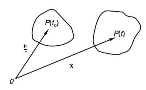
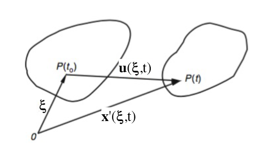
“Particle” at point $\boldsymbol{\xi}$ at a reference time $t_0$, moves to point $\mathbf{x}'$ at a later time t. Field P is described as a function of $\boldsymbol{\xi}$ and t.

In the spatial description, the behaviour of the body is observed at fixed points in space over time, rather than tracking the individual particles or elements in the fluid. Imagine placing an imaginary grid or network of points throughout the fluid and analyse how the fluid properties, such as velocity, pressure, and density, vary at each point in the grid as time progresses. This is often the preferred description for fluids.

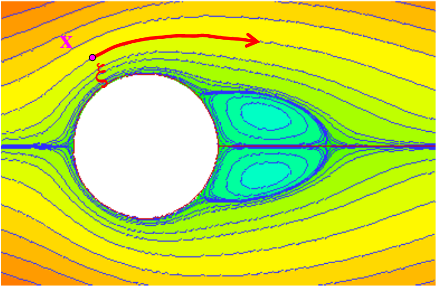
In the example flow, velocity at point $\mathbf{x}$, does not change with time, but velocity that a particle originally in the same position $\xi$ experiences with time does change.

Material Time Derivative #

The time derivative is the rate of change (with time) of a quantity for a material particle.

In the material description , the time derivative of P is: $\hspace{0.1cm} \large{\frac{DP}{Dt}} = \Bigl(\frac{\partial P}{\partial t}\Bigr)_\xi \hspace{2cm}$ Note here P($\boldsymbol{\xi}, t$)

In the spatial description , the time derivative of P is: $\hspace{0.1cm} \large{\frac{DP}{Dt}} = \Bigl(\frac{\partial P}{\partial t}\Bigr)_\xi = \Bigl(\frac{\partial P}{\partial t}\Bigr)_x + \frac{\partial P}{\partial t_i} \Bigl(\frac{\partial x'_i}{\partial t}\Bigr)_\xi \hspace{1cm}$ Note here P($\mathbf{x}, t$)

where $\large{\Bigl(\frac{\partial \mathbf{x}'}{\partial t}\Bigr)_\xi}= \frac{D\mathbf{x}}{Dt}$ where the velocity of the particle is denoted by $\xi$.
$\hspace{1cm} \mathit{Material} \hspace{0.7cm} \mathit{Spatial} $

\[ \frac{DP}{Dt} = \frac{\partial P}{\partial t} + \mathbf{v} \cdot \nabla P \]

This definition works in any coordinate frame.

Example: Acceleration #

In the spatial description: $ \large{\mathbf{a}} = \frac{D\mathbf{v}}{Dt} = \frac{\partial v}{\partial t} + \mathbf{v} \cdot \nabla \mathbf{v}$

Let’s determine the acceleration of a particle in a given spatial velocity field, in 2-D, i.e., $i$ takes on the values 1,2.

\[ v_i = \frac{kx_i}{(1 + kt)} \]

For $a_1$:

\[ \frac{\partial v_1}{\partial t} = -\frac{kx_1 (k)}{(1 + kt)^2} = -\frac{k^2 x_1}{(1 + kt)^2} \]

\[ v_1 \frac{\partial v_1}{\partial x_1} = \frac{kx_1}{(1 + kt)} \frac{k}{(1 + kt)} = \frac{k^2 x_1}{(1 + kt)^2} \]

\[ v_2 \frac{\partial v_1}{\partial x_2} = 0 \]

Hence:

\[ a_1 = \frac{Dv_1}{Dt} = \frac{\partial v_1}{\partial t} + v_1 \frac{\partial v_1}{\partial x_1} = -\frac{k^2 x_1}{(1 + kt)^2} + \frac{k^2 x_1}{(1 + kt^2)} = 0 \]

\[ \text{Velocity Field at} \hspace{0.1cm} t = 0 \hspace{0.1cm} (k = 1) \]

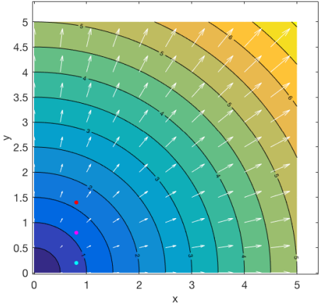
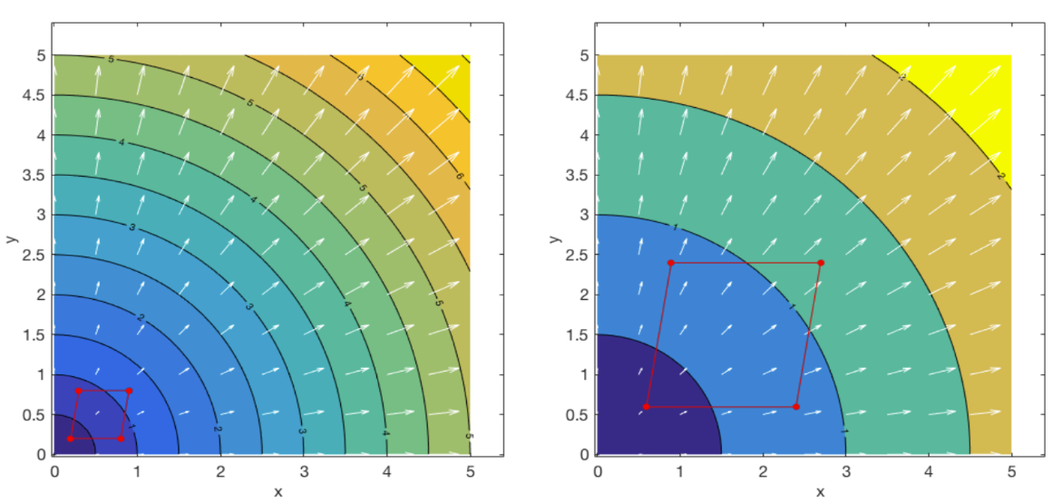
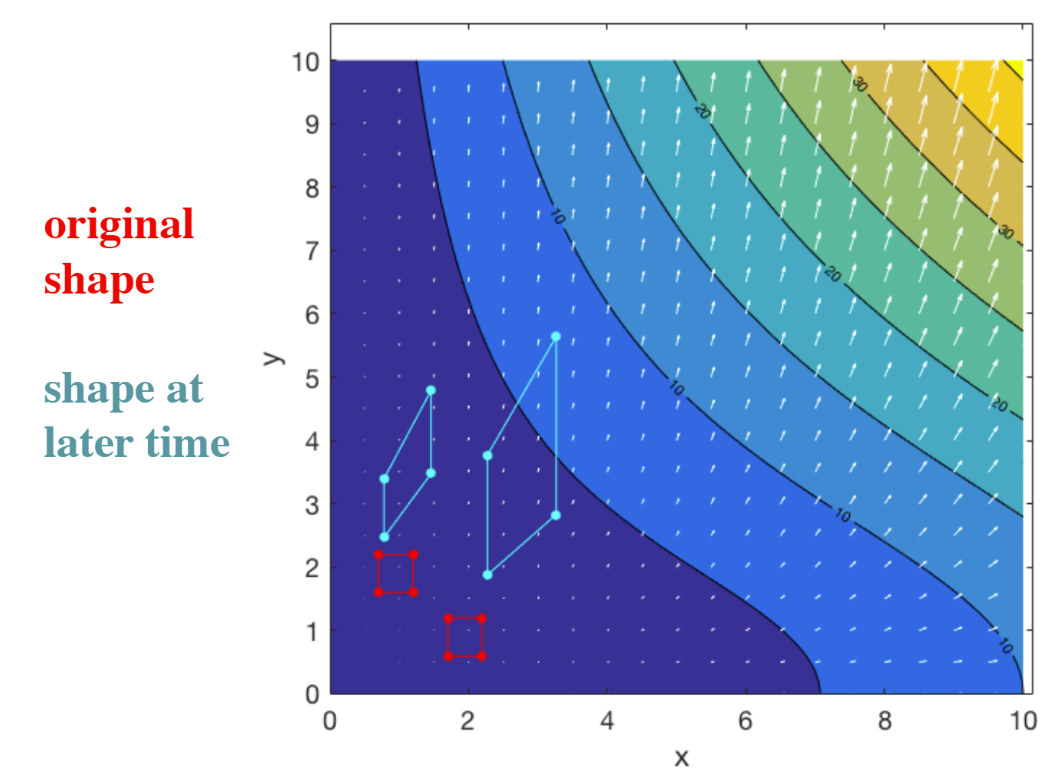
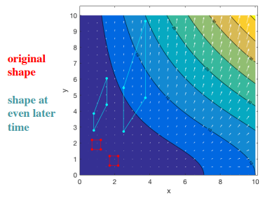
2D velocity field with contours for magnitude, and arrows showing direction and magnitude. Three coloured markers are inserted in the field at $t$=0

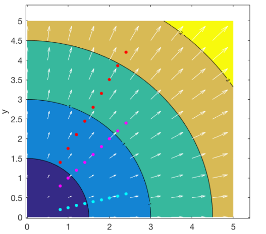
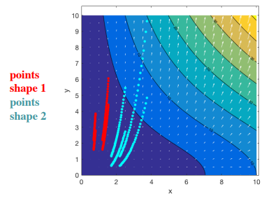
\[ \text{Spatial velocity field}: \hspace{0.2cm} {v_i} = \frac{kx_i}{1 + kt} \hspace{2cm} \text{Acceleration}: \hspace{0.2cm} {a_i} = \frac{Dv_i}{Dt} = \frac{\partial v_i}{\partial t} + v_j \frac{\partial v_i}{\partial x_j} = 0 \]

\[ \text{Velocity Field at } t = 2 \hspace{0.1cm} (k = 1) \]

Same velocity field as in the previous figure, but now shown at $t$=2. The evolution of the marker positions is shown at constant time intervals between [0:2]

Note that with this expression for the full material acceleration, Newton’s second law:

\[ \mathbf{F} = m \mathbf{a} \hspace{0.1cm} \text{or per unit volume }\mathbf{f} = \rho \mathbf{a} \hspace{0.1cm} \]

becomes: $$ {\mathbf{f}} = \rho \frac{D \mathbf{v}}{Dt} = \rho \Biggl(\frac{\partial \mathbf{v}}{\partial t} + \mathbf{v} \cdot \nabla \mathbf{v}\Biggr) $$

Displacement #

Displacement of a body can result in rigid body motion or deformation of the body.

Pathlines #

Motion of a continuum can be described by: path lines $\mathbf{x}' = \mathbf{x}'(\boldsymbol{\xi}, t)$ or by displacement fields $\mathbf{u}(\xi, t) = \mathbf{x}'(\boldsymbol{\xi}, t) - \boldsymbol{\xi}$ .

Let’s determine the pathline for the $x'_1$ component of the particle’s position for the spatial velocity field of the earlier acceleration example.

\[ v_i = \frac{kx_i}{1 + kt} \]

We can see that:

\[ v_i = \frac{\partial x'_i}{\partial t} = \frac{kx_i}{1 + kt} \]

\[ \int_{\xi_i}^{x'_i} \frac{1}{kx_i} dx_i = \int_{0}^{1} \frac{1}{1 + kt} dt \]

\[ \frac{1}{k} [\ln x'_i - \ln \xi_i] = \frac{1}{k}[\ln(1 + kt) - \ln(1)] \]

\[ x'_i(\xi, t) = (1 + kt)\xi_i \]

From this we can see that:

\[ \text{Material displacement field}: \hspace{0.2cm} u'_i = kt\xi_i \hspace{1.5cm} \text{Material velocity field}: \hspace{0.2cm} v'_i = v_i = k\xi_i \]

Rigid Body Motion #

The motion through which a body as a whole shifts from one point to another is known as a translation . When a rigid body moves in a translational motion, the line segment between any two particles of the body remains parallel.

\[ \mathbf{x}' = \boldsymbol{\xi} + \mathbf{c}(t), \text{with } \mathbf{c}(0) = 0 \]

\[ \Rightarrow \mathbf{u}'(t) = \mathbf{x}(t) - \boldsymbol{\xi} = \mathbf{c}(t) \]

In the case of rigid body motion, the displacement is the same for each point, i.e. $\mathbf{c}(t)$ does not depend on $\mathbf{x}$.

Rotation is a rigid body motion when a solid body moves in a circular path around a fixed point or fixed axis. It is represented mathematically by:

\[ \mathbf{x' - b} = \mathbf{R}(t)(\boldsymbol{\xi} - \mathbf{b}) \]

Where $\mathbf{R}(t)$ is the rotation tensor, with $\mathbf{R(0) = I}$, $\mathbf{b}$ is the point of rotation. $\mathbf{R}(t)$ is an orthogonal transformation, meaning it preserves the lengths and angles of the body. ($\mathbf{R^T R = I}, \text{det}(\mathbf{R}) = 1)$.

If $\mathbf{u}$ depends on both $\mathbf{x}$ and $\mathbf{t}$, then the body will undergo internal deformation.

Example: Displacement #

Let’s look at the velocity field from earlier. ${v_i} = \frac{kx_i}{1 + kt}$

\[ t = 0 \hspace{7.5cm} t = 2 \]

We can see that the shape positioned in this velocity field undergoes both translation and deformation.

Deformation Tensor #

For small dr

\[ P_1 \hspace{0.2cm} \text{at} \hspace{0.2cm} \mathbf{r} \Rightarrow P'_1 \hspace{0.2cm} \text{at} \hspace{0.2cm} \mathbf{r + u(r)} \]

\[ P_2 \hspace{0.2cm} \text{at} \hspace{0.2cm} \mathbf{r + dr} \Rightarrow P'_2 \hspace{0.2cm} \text{at} \hspace{0.2cm} \mathbf{r + dr + u(r + dr)} \]

\[ \mathbf{dr}' = P_2 - P_1 = \mathbf{dr + [u(r + dr) - u(r)] = dr + du(r) = dr + dr \cdot \nabla u(r)} \]

\[ \text{Deformation of} \hspace{0.1cm} P_2 \hspace{0.1cm} - \hspace{0.1cm} P_1 \hspace{0.1cm} \text{described by} \hspace{0.1cm} du_i = dx_j \frac{\partial u_i}{\partial x_j} \]

\[ \mathbf{du = dr \cdot \nabla u = \nabla^T u \cdot dr} \]

\[\begin{split} {du_i} = dx_j \frac{\partial u_j}{\partial x_j}\hspace{0.2cm} : \hspace{1cm} \begin{pmatrix} du_1 \\ du_2 \\ du_3 \\ \end{pmatrix} = \begin{pmatrix} dx_1 & dx_2 & dx_3 \\ \end{pmatrix} \begin{bmatrix} \frac{\partial u_1}{\partial x_1} & \frac{\partial u_2}{\partial x_1} & \frac{\partial u_3}{\partial x_1} \\ \frac{\partial u_1}{\partial x_2} & \frac{\partial u_2}{\partial x_2} & \frac{\partial u_3}{\partial x_2} \\ \frac{\partial u_1}{\partial x_3} & \frac{\partial u_2}{\partial x_3} & \frac{\partial u_3}{\partial x_3} \\ \end{bmatrix} \end{split}\]

\[ {\frac{\partial u_i}{\partial x_j}} = \frac{1}{2} \Biggl(\frac{\partial u_i}{\partial x_j} + \frac{\partial u_j}{\partial x_i}\Biggr) + \frac{1}{2} \Biggl(\frac{\partial u_i}{\partial x_j} + \frac{\partial u_j}{\partial x_i}\Biggr) \]

\[ {\nabla \mathbf{u = \color{red}{\frac{1}{2} (\nabla u + \nabla u^T)} + \color{purple}{\frac{1}{2} (\nabla u - \nabla u^T)}}} \]

\[ {\hspace{1cm} \color{red}{\varepsilon_{ij}} \hspace{4cm} \color{purple}{\omega_{ij}}} \]

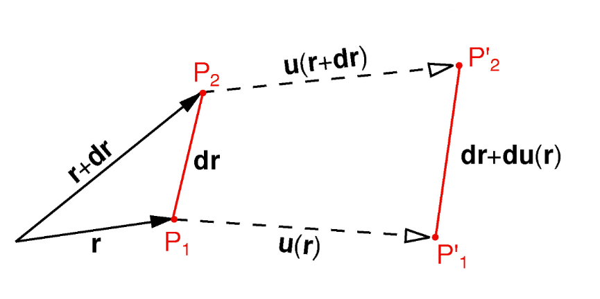
Total deformation is:

Rigid body transformation - $\mathbf{u(r)}$
Rigid body rotation - $\mathbf{\color{purple}{\omega} \hspace{0.1cm} dr}$
Internal deformation, strain - $\mathbf{\color{red}{\varepsilon} \hspace{0.1cm} dr}$ - Result of stresses

Infinitesimal Strain and Rotation Tensors #

3D, Cartesian representations:

\[\begin{split} \large{\color{red}{\varepsilon}} = \begin{bmatrix} \frac{\partial u_1}{\partial x_1} & \frac{1}{2} \Biggl(\frac{\partial u_2}{\partial x_1} + \frac{\partial u_1}{\partial x_2}\Biggr) & \frac{1}{2} \Biggl(\frac{\partial u_3}{\partial x_1} + \frac{\partial u_1}{\partial x_3}\Biggr) \\ \frac{1}{2} \Biggl(\frac{\partial u_1}{\partial x_2} + \frac{\partial u_2}{\partial x_1}\Biggr) & \frac{\partial u_2}{\partial x_2} & \frac{1}{2} \Biggl(\frac{\partial u_3}{\partial x_2} + \frac{\partial u_2}{\partial x_3}\Biggr) \\ \frac{1}{2} \Biggl(\frac{\partial u_1}{\partial x_3} + \frac{\partial u_3}{\partial x_2}\Biggr) & \frac{1}{2} \Biggl(\frac{\partial u_2}{\partial x_3} + \frac{\partial u_3}{\partial x_2}\Biggr) & \frac{\partial u_3}{\partial x_3} \\ \end{bmatrix} \end{split}\]

\[\begin{split} \large{\color{purple}{\omega}} = \begin{bmatrix} 0 & \frac{1}{2} \Biggl(\frac{\partial u_2}{\partial x_1} - \frac{\partial u_1}{\partial x_2}\Biggr) & \frac{1}{2} \Biggl(\frac{\partial u_3}{\partial x_1} - \frac{\partial u_1}{\partial x_3}\Biggr) \\ \frac{1}{2} \Biggl(\frac{\partial u_1}{\partial x_2} - \frac{\partial u_2}{\partial x_1}\Biggr) & 0 & \frac{1}{2} \Biggl(\frac{\partial u_3}{\partial x_2} - \frac{\partial u_3}{\partial x_2}\Biggr) \\ \frac{1}{2} \Biggl(\frac{\partial u_1}{\partial x_3} - \frac{\partial u_3}{\partial x_1}\Biggr) & \frac{1}{2} \Biggl(\frac{\partial u_2}{\partial x_3} - \frac{\partial u_3}{\partial x_2}\Biggr) & 0 \\ \end{bmatrix} \end{split}\]

Diagonal Infinitesimal Strain Tensor Elements #

For a line segment $\mathbf{dr} = (dx_1, 0, 0)$ deforming in a displacement field $ \mathbf{u} = (u_1, 0, 0) $

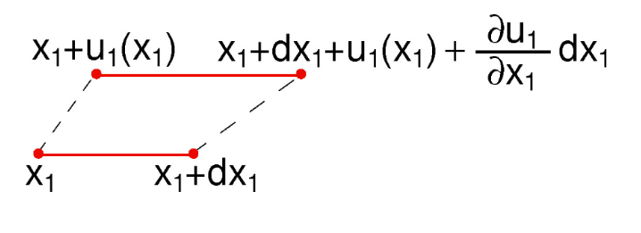
The new length: $ dx'_1 \approx dx_1 + (\partial u_1 / \partial x_1 )dx_1 = dx_1 + \varepsilon_{11} dx_1$

\[ \Rightarrow {\varepsilon_{11}} = [dx'_1 - dx_1]/dx_1 \]

\[ \varepsilon_{11} \text{ represents the relative change in length of a line, element, originally in the} \hspace{0.1cm} x_1 \hspace{0.1cm} \text{direction} \]

We can similarly find the relative change in volume $(V' - V)/V$ of a cube $V =dx_1 dx_2 dx_3$

The length of each side of the cube changes from $dx_i$ to $dx_i (1+\varepsilon_{ii})$.

Neglecting any terms in higher orders of $\varepsilon_{ii}$, the new volume becomes

\[ V' \approx (1+ \varepsilon_{11} + \varepsilon_{22} + \varepsilon_{33}) dx_1 dx_2 dx_3\]

That is, the fractional change in volume $$ dV/V \approx \varepsilon_{11} + \varepsilon_{22} + \varepsilon_{33} = \varepsilon_{ii} = \text{tr}(\varepsilon) = \nabla \cdot \mathbf{u} $$

Off-Diagonal Infinitesimal Strain Tensor Elements #

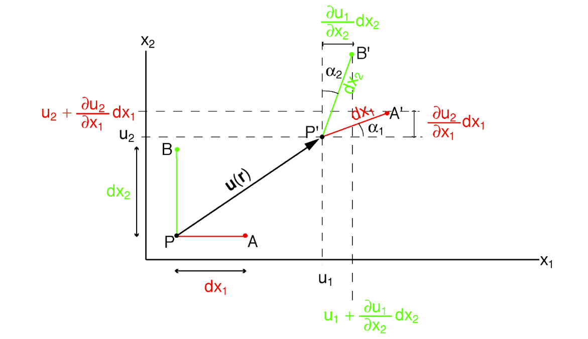
\[\begin{split} \varepsilon_{12} = \varepsilon_{21} = \frac{(\alpha_1 + \alpha_2)}{2} \hspace{0.5cm} {\begin{cases} \alpha_1 \approx \sin \alpha_1 = \frac{(\partial u_2/\partial x_1) dx_1}{dx_1} = \frac{\partial u_2}{\partial x_1} \\ \alpha_2 \approx \frac{(\partial u_1/ \partial x_2) dx_2}{dx_2} = \frac{\partial u_1}{\partial x_2} \\ \end{cases}} \end{split}\]

$2 \varepsilon_{12}$ is the change in angle between $dx_1$ and $dx_2$, orginally 90 degrees .

Infinitesimal Rotation Tensor Elements #

Diagonal elements of $\boldsymbol{\omega}$ are equal to 0. Off-diagonal elements:

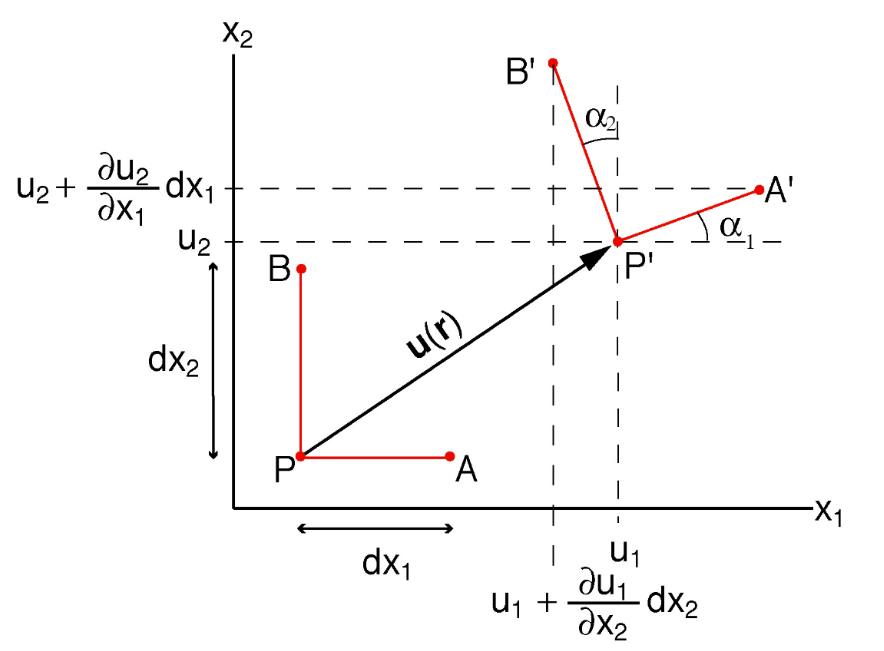
\[ {\omega_{12}} = - \hspace{0.1cm} \omega_{21} = \Biggl[\frac{(\partial u_2/\partial x_1) - (\partial u_1/\partial x_2)}{2}\Biggr] = \frac{(\alpha_1 - \alpha_2)}{2} \]

$\omega_{12}$ is the common rigid rotation angle of vectors in the $dx_1 - dx_2$ plane (around $x_3$).

$\color{orange}{\text{Extra}}$: Rotation tensor and Rotation vector #

For an antisymmetric tensor W, a corresponding dual or axial vector w can be found such that:

\[ \mathbf{W \cdot a = w \times a} \]

Vector $\mathbf{w}$ relates to the component of $\mathbf{W}$ as:

\[ \mathbf{w} = - W_{23} \mathbf{\hat{e}_1} + W_{13} \mathbf{\hat{e}_2} - W_{12} \mathbf{\hat{e}_3} \]

For the rotation tensor, an equivalent rotation vector exists:

\[ \mathbf{\omega \cdot dx} = r_\omega \times \mathbf{dx} \hspace{1cm} \text{where} \hspace{1cm} r_\omega = \frac{1}{2} \nabla \times \mathbf{u} \]

Note that $\omega$ only describes the overall rigid body roation, not the total rotation of each individual segment dx, which is also influenced by $ \varepsilon $.

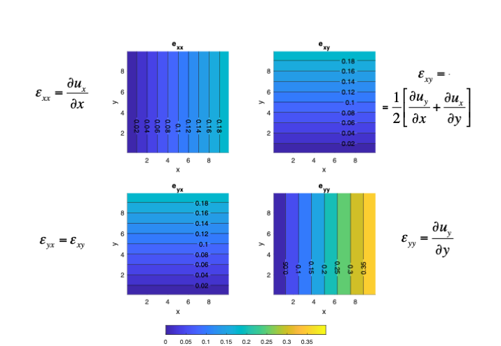
Example Displacement - Infinitesimal Strain #

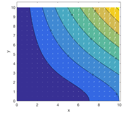
Displacement:

\[ u_x = 0.1 x^2 \hspace{0.5cm} u_y = 0.4 xy \]

Displacement gradients can be visualised as follows:

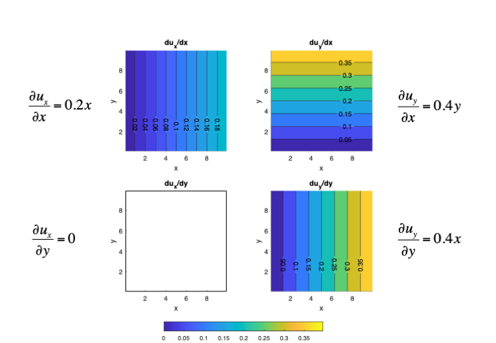
We can then find the strain elements by:

\[ \varepsilon_{xx} = \frac{\partial u_x}{\partial x} \hspace{1.5cm} \varepsilon_{yx} = \varepsilon_{xy} = \frac{1}{2} \Bigl[\frac{\partial u_y}{\partial x} + \frac{\partial u_x}{\partial y}\Bigr] \hspace{1.5cm} \varepsilon_{yy} = \frac{\partial u_y}{\partial y} \]

And in graphical form:

The deformation after the finite strain can be shown graphically as:

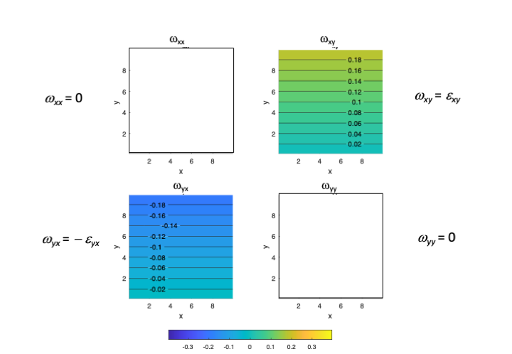
Additionally, we can calculate the infinitesimal rotation elements:

\[ \omega_{xx} = 0 \hspace{1.5cm} \omega_{yy} = 0 \hspace{1.5cm} \omega_{xy} = -\hspace{0.1cm}\omega_{yx} = \frac{1}{2} \Bigl[\frac{\partial u_y}{\partial x} - \frac{\partial u_x}{\partial y}\Bigr] \]

And display them graphically:

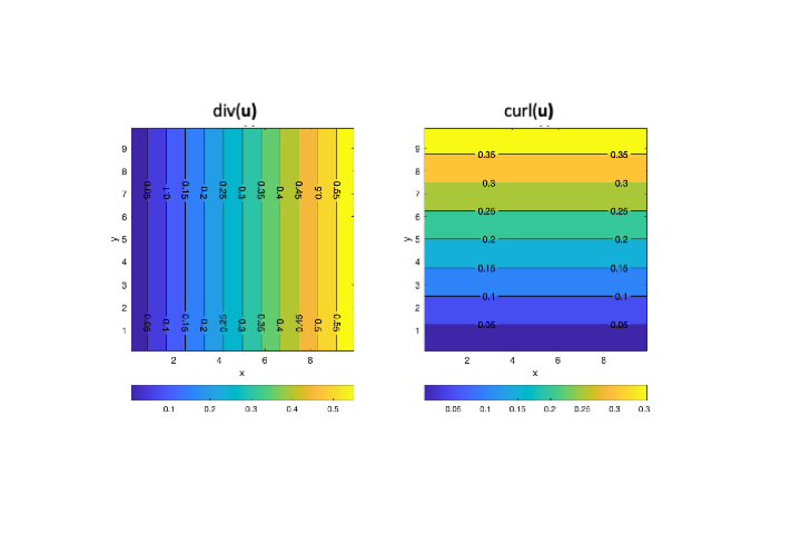
We can similarly find the divergence and curl of the velocity field:

\[ \nabla \cdot \mathbf{u} = \frac{\partial u_x}{\partial x} + \frac{\partial u_y}{\partial y} \hspace{2.2cm} \nabla \times \mathbf{u} = \Bigl(\frac{\partial u_x}{\partial x} + \frac{\partial u_y}{\partial y} \Bigr) \]

Infinitesimal Strain Tensor Properties #

Similarly to the stress tensor, we can transform the strain tensor to an arbitrary coordinate frame:

\[ \varepsilon_{nn} = \varepsilon_{11} \cos^2{\phi} + \varepsilon_{12} \sin{\phi}\cos{\phi} + \varepsilon_{21} \sin{\phi}\cos{\phi} + \varepsilon_{12} \sin^2{\phi} \]

\[ \varepsilon_{ns} = \varepsilon_{11} \sin{\phi}\cos{\phi} + \varepsilon_{21} \sin^2{\phi} - \varepsilon_{12} \cos^2{\phi} - \varepsilon_{22} \sin{\phi} \cos{\phi} \]

$ \varepsilon_1, \hspace{0.1cm} \varepsilon_2, \hspace{0.1cm} \varepsilon_3 $ represent the principal strains. These are the maximum and minimum length changes of an elemental volume.
$ \text{tr}(\boldsymbol{\varepsilon}) = \theta $ is the sum of the normal strains and is equal to the volume change.
The deviatoric strain $ \varepsilon'_{ij} = \varepsilon_{ij} - \frac{\theta}{3} \delta_{ij} $. This strain represents a change in shape of the object, and no change in volume.
$\text{tr}(\boldsymbol{\varepsilon}') = 0$, does not imply that $ \varepsilon'_{ij}$ = 0 for $ i = j $.
$\varepsilon_{ij} = 0$ for $i = j$ does not ensure no shape change.

Strain Elements #

\[\begin{split} \boldsymbol{\varepsilon} = \begin{bmatrix} \varepsilon_{11} & \varepsilon_{12} & \varepsilon_{13} \\ \varepsilon_{21} & \varepsilon_{22} & \varepsilon_{23} \\ \varepsilon_{31} & \varepsilon_{32} & \varepsilon_{33} \\ \end{bmatrix} \end{split}\]

\[ \mathbf{\hat{e}_1 \cdot \boldsymbol{\varepsilon} \cdot \hat{e}_1} = \varepsilon_{11} \]

\[ \mathbf{\hat{e}_1 \cdot \boldsymbol{\varepsilon} \cdot \hat{e}_2} = \varepsilon_{12} \]

$\mathbf{ \boldsymbol{\varepsilon} \cdot \hat{p} = dp'}$ is the change in the unit vector $\mathbf{\hat{p}}$ after the deformation by $\boldsymbol{\varepsilon}$.

$\mathbf{\hat{p}} \cdot \boldsymbol{\varepsilon} \cdot \mathbf{\hat{p}}$ is the elongation by $\boldsymbol{\varepsilon}$ of the unit vector $\mathbf{\hat{p}}$ in the direction $\mathbf{\hat{p}}$

Which is the same as $\mathbf{\hat{p} \cdot dp' = |dp'| \cos{\alpha}}$.

Strain Rate Tensor #

In a similar way as a strain tensor, a tensor that describes the rate of change of deformation can be defined from the velocity gradient.

\[ \frac{D}{Dt}\mathbf{dr} = \nabla \mathbf{v} \]

\[\begin{split} \large{\nabla} \mathbf{v} = \begin{bmatrix} \frac{\partial v_1}{\partial x_1} & \frac{\partial v_2}{\partial x_1} & \frac{\partial v_3}{\partial x_1} \\ \frac{\partial v_1}{\partial x_2} & \frac{\partial v_2}{\partial x_2} & \frac{\partial v_3}{\partial x_2} \\ \frac{\partial v_1}{\partial x_3} & \frac{\partial v_2}{\partial x_3} & \frac{\partial v_3}{\partial x_3} \end{bmatrix} \end{split}\]

\[ \nabla \mathbf{v} = \color{red}{\frac{1}{2} (\nabla \mathbf{v} + \nabla \mathbf{v}^T)} + \color{purple}{\frac{1}{2} (\nabla \mathbf{v} - \nabla \mathbf{v}^T)} \]

\[ \nabla \mathbf{v = \color{red}{D} + \color{purple}{W}} \]

The velocity gradient tensor is the sum of the $\color{red}{\text{strain rate}}$ and $\color{purple}{\text{vorticity}}$ tensors.

Over small increments, we can assume that a constant displacement gradient is encountered.

Practise #

Do exercises $\color{blue}{\textbf{1, 2, 5, 7, 9a}}$:

Additional practise $\color{green}{\textbf{3, 6, 8}}$:

Advanced oractise $\color{orange}{\textbf{4, 9b, 10}}$: