2.1 Stress and Tensors #
Lecture 2.1 & 2.2
Saskia Goes, s.goes@imperial.ac.uk
Table of Contents#
Outline #
Part 1: Stress and Tensors#
Cauchy Stress Tensor
(Stress) tensor symmetry
Coordinate transformation (stress) tensors
Shear and normal stresses
Tensor invariants
Learning outcomes #
Understand the meaning of different components of 3D Cauchy stress tensor
Know how to determine state of stress on given plane
Be able to decompose a rank 2 tensor into symmetric and anti-symmetric components
Be able to transform rank 2 tensor to a new basis
Be able to determine shear and normal stresses on a plane
Cauchy Stress#
The Cauchy stress tensor is a second-order tensor that completely defines the state of stress at a point inside a material in its deformed state. It is used for the stress analysis of materials undergoing small deformations, whereas for large deformations other methods have to be used such as the Piola-Kirchhoff stress tensor.
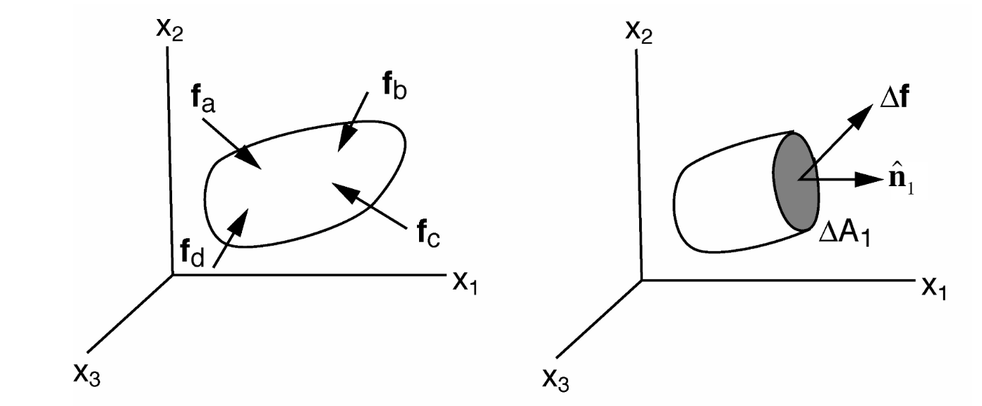
Consider a body that subject to a set of forces (body and surface forces) (see figure above). These put this body in a state of stress. We can evaluate this state of stress by considering a planar cut through the body and evaluate the traction (also called stress vector) that represents the net force on this plane.
If we take a plane with a normal in \(x_1\) direction, i.e. with a normal \(\mathbf{\hat{n}}_1\), then this traction vector \(\mathbf{t}_1\) is:
The traction has three components, which we will denote \(\sigma_{11},\sigma_{12},\sigma_{13}\):
To fully describe the stress in all directions, we will need the tractions, \(\mathbf{t}_1, \mathbf{t}_2, \mathbf{t}_3\) on each of the planes with normals in the principal coordinate directions, giving a total of nine stress components:
The first index (j) describes the orientation of the plane (\(\mathbf{\hat{n}}_j\)), whereas the second index (i) describes the orientation of the force (\(i\)-th component of \(\mathbf{t}\). However are nine components sufficient?
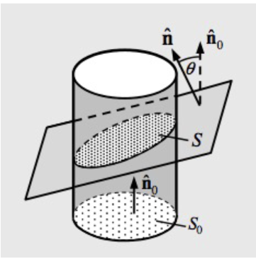
Plane area as a vector #
The area of plane S can be defined in terms of vectors, assuming that \(S_0\) and \(\theta\) are known.
How many stress tensor components?#
Let us now try to answer whether nine components are sufficient to capture all the stresses acting on an object.
We can demonstrate this by taking the equilibrium for a tetrahedron.
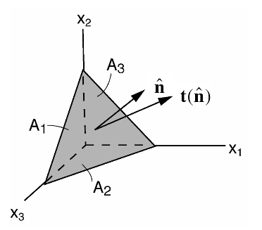
Given the stresses acting on surfaces \(A_1, A_2 \; \text{and} \; A_3\). Find \(\mathbf{t(\hat{n})}. \)
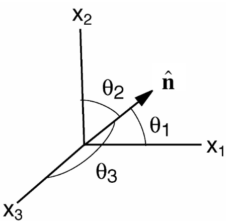
The normals and areas of each of these surfaces are:
Taking equilibrium gives:
This gives :
and similarly
So indeed the nine stress components are enough to completely describe the three components of a traction vector \(\mathbf{t}\) on a arbitrarily oriented plane with normal \(\mathbf{\hat{n}}\). In index notation, the three equations above can be summarised as:
This final expression uses the Einstein convention.
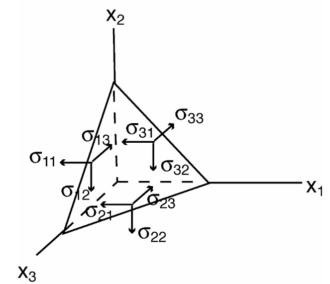
3-D Stress State #
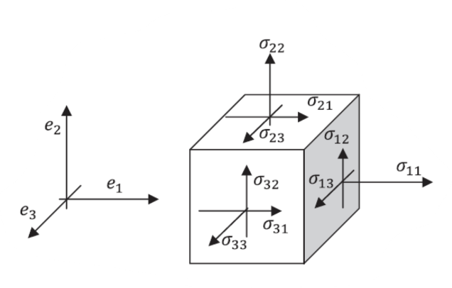
The first index of the stress tensor represents the orientation of the plane whereas the second index represents the orientation of the force.
The force is considered positive in the direction of the normal (as shown).
Note the unusual index order, j before i, to reflect that multiplication involves the transpose of \(\sigma\)
In matrix notation, this gives:
Important Points#
t and \(\mathbf{\hat{n}}\) are tensors of rank 1 (i.e vectors) and \(\bar{\bar{\sigma}}\) is a tensor of rank 2 in 3-D.
Compressive stresses have a negative sign whereas tensile forces have a positive sign.
The diagonal elements of the matrix (i.e when \(i = j\)) are normal stresses and the off-diagonal elements (i.e when \(i \neq j\)) are shear stresses.
Rank 2 tensors can be written as square matrices and have algebraic properties similar to matrices.
Tensor Symmetry #
A tensor can be symmetric in 1 or more indices.
For example, a rank 2 tensor is symmetric if: \(S_{ij} = S_{ji} \Rightarrow \mathbf{S} = \mathbf{S^T}\),
and vice versa, a rank 2 tensor is anti-symmetric if: \(S_{ij} = - S_{ji} \Rightarrow \mathbf{S} = - \mathbf{S^T}\).
For tensors of higher rank: \(S_{ijk} = S_{jik}\) for all \(i,j,k\) \(\Rightarrow\) means \(\mathbf{S}\) is symmetric in \(i,j\).
Given \(n\) is the dimension of the tensor:
For an antisymmetric \(\mathbf{T}\) of rank 2 (with \(T_{ij} = 0, \text{for } i = j\)), the number of independent components is given by : \( {\frac{n(n-1)}{2}} \).
For a symmetric \(\mathbf{T}\) of rank 2, the number of independent components is given by : \( {\frac{n(n+1)}{2}} \)
Any tensor \(\mathbf{T}\) of rank 2 can be decomposed into its symmetric and antisymmetric parts:
Symmetry of the Stress Tensor #
Consider a cube with dimensions \({\Delta}x_1\), \({\Delta}x_2\) and \({\Delta}x_3\)
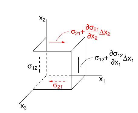
We can see from the figure above that the following stresses acting on the \({x_2}\)-\({x_3}\) plane form a force couple that can induce a rotational moment around the \(x_3\) axis, with moment arm \({\frac{\Delta x_1}{2}}\).
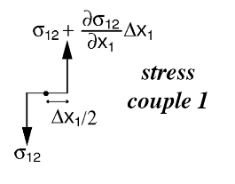
Similarly, the stresses acting on the \(x_1\)-\(x_3\) planes form a couple that can induce a rotational moment around the \(x_3\) axis, with moment arm \(\frac{\Delta x_2}{2}\).
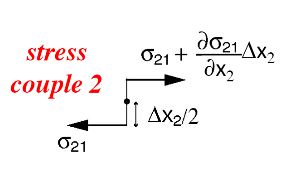
Assuming static equilibrium, we can take a balance of the moments inducing rotation in the \(x_3\) direction. This gives:
Similarly, balancing \(m_1\) and \(m_2\), gives:
Thus, the stress tensor is symmetric.
Transformations of Tensors #
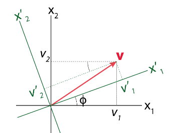
Remember from Lecture 1.2 that the physical quantities should not depend on the coordinate frame. We derived vthere the transformation law for vectors on a Cartesian orthonormal basis. Tensors follow the same linear transformation laws.
For vectors on an orthonormal basis:
Coefficients \(\alpha_{ij}\) depend on the angle \(\phi\) between \(x_1\) and \( x'_1\) (or \(x_2\) and \( x'_2\)).
In order to transform our stresses from one coordinate system to another, remember that the relation between the stress vector, stress tensor and plane normal needs to hold in any coordinate system.
We want to find a relation between \(\sigma'\) and \(\sigma\).
Using the relations for transforming vectors to a new coordinate system:
We also need to remember that transformation matrices are orthogonal. That is:
and:
The transformation for our stress tensor follows:
Because: $\( \mathbf{t'} = \boldsymbol{\sigma}'^\text{T} \mathbf{\hat{n}'} \)$
This means that: $\( \boldsymbol{\sigma}'^\text{T} = \color{blue}{\text{A}} \boldsymbol{\sigma}^\text{T} \color{red}{\text{A}^\text{T}} \)$
Using index notation:Each dependence that the tensor has on direction transforms as a vector, therefore two transformations are required.
In general:
An n-dimensional tensor \(\mathbf{T}\) of rank r consists of \(\mathit{n^r}\) components.
Such a tensor \(\text{T}_{i1, i2,...in}\) is defined relative to the basis of the real, linear, n-dimensional space \(\mathbf{S}_n\).
Under a coordinate transformation, \(\mathbf{T}\) transforms as: \(T'_{ij...n} = \alpha_{ip} \alpha_{jq} \alpha_{nt} \mathbf{T}_{pq...t}\) (i.e one transformation per rank).
For orthonormal bases, the matrices \(\alpha_{ik}\) are orthogonal transformations, i.e \(\alpha_{ik}^{-1} = \alpha_{ki}\) (i.e., \(\mathbf{A} = \mathbf{A}^T\); columns and rows are orthogonal and have length = 1). If the basis is Cartesian, \(\alpha_{ik}\) are real.
Transforming the 2-D stress tensor #
This process lets us determine the normal and shear stress on a plane.
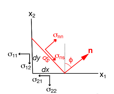
We can see above that the force normal to the plane is:
Therefore the normal stress on the plane is:
This gives:
And similarly the shear stress is given by:
Mutiplying this out (Verify this yourself) gives:
This is equivalent to the tensor transformation.
Writing out the full transformation, we know that:
Therefore in the case of a stress tensor:
In tensor notation:
In matrix notation:
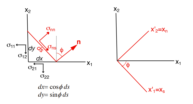
For \(\hat{x}_1 = (1,0),\hspace{0.1cm} \hat{x}_2 = (0,1),\hspace{0.1cm} \hat{x}'_1 = (\cos{\phi},-\sin{\phi}) \hspace{0.5cm} \hat{x}'_2 = (\sin{\phi},\cos{\phi})\).
The first row of \(\text{A}\) consists of \(\hat{x}'_1\) and the second row consists of \(\hat{x}'_2\).
You may recognise \(\text{A}\) as a matrix that describes an anticlockwise rigid-body rotation over an angle \(\phi\).
\(\text{A}^\text{T}\) describes a clockwise rotation over an angle \(\phi\). The first column of \(\text{A}^\text{T}\) consists of \(\hat{x}'_1\) and the second column of \(\hat{x}'_2\).
Diagonalising/Principal Stresses#
Real-valued, symmetric rank 2 tensors (square, symmetric matrices) can only be diagonalised, i.e a coordinate frame can be found, such that only the diagonal elements (normal stresses) remain.
For the stress tensor, these elements \(\sigma_1 ,\sigma_2, \sigma_3\) are called the principal stresses.
\(\color{orange}{\text{Extra:}}\) Note that the method for finding principal stresses and their directions is advanced content
Such a transformation can be cast as:
where \(\mathbf{x_i}\) are eigenvectors or characteristic vectors and \(\lambda_i\) are the eigenvalues, characteristic or principal values.
Note that a non-trivial solution exists only if \(\text{det}(\mathbf{T - \lambda I}) = 0\).
Stress/Tensor Invariants#
Invariants are properties of a tensor that do not change if the coordinate system is changed.
A rank-2 tensor has three invariants. For a symmetric tensor these are:
These invariants are important in operations such as diagonalising.
Hydrostatic and Deviatoric Stress#
Each stress element in the stress tensor can be split into two components, the hydrostatic stress and the deviatoric stress.
$ \text{tr}(\sigma) $ is the trace of the stress tensor and is equal to the sum of the normal stresses ( $\sigma_{11} + \sigma_{12} + \sigma_{13}$ ). This is also an invariant of the tensor.
The hydrostatic stress is the stress that leads to volume change.
\(\sigma_{ij}'\) is the deviatoric stress \( = \sigma_{ij} + P\delta_{ij}\). This is the stress that leads to shape change.
Note that in geological applications \(\sigma_{ij}' \neq \sigma_{ij} + \rho g z \delta_{ij}\)