1.2 Vector Transformations

Lecture 1.2
Saskia Goes, s.goes@imperial.ac.uk

Table of Contents

Learning outcomes

1. Perform transformation of a vector from one Cartesian basis to another

2. Be able to do basic vector/tensor calculus (time and space derivatives, divergence, curl of a vector field) on these bases

Vector Transformation

Vector magnitude and direction do not depend on basis.

When defined on an orthonormal basis, like rectangular Cartesian, the transformation to other orthonormal basis is simple, with real coefficients.

\[ \hat{e}_i \cdot \hat{e}_j = 0 \hspace{1cm} \text{if i} \neq \text{j} \]

\[ \hat{e}_i \cdot \hat{e}_i = |\hat{e}_i| = 1 \]

Check out Khan Academy lectures on orthonormal bases for more information.

Physical parameters should not depend on coordinate frame.

For vectors on an orthonormal basis, the transformed vector v’ depends on v:

\[ \text{v'}_1 = \alpha_{11} \text{v}_1 + \alpha_{12} \text{v}_2 \]

\[ \text{v'}_2 = \alpha_{21} \text{v}_1 + \alpha_{22} \text{v}_2 \]

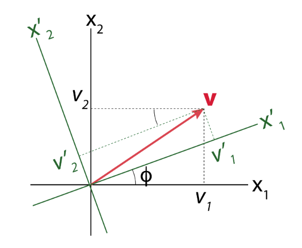
Coefficients \(\alpha_{ij}\) depend on angle \(\phi\) between \(\text{x}_1\) and \(\text{x'}_1\) (or \(\text{x}_2\) and \(\text{x'}_2\))

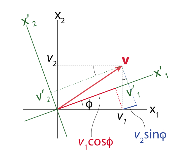
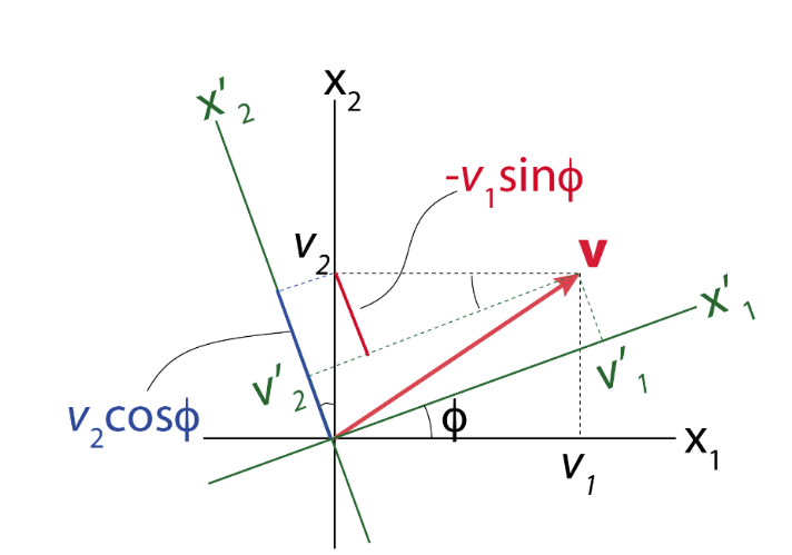
From the figures above, we can deduce that:

\(\hspace{6cm} \text{v'}_1 = \cos{\phi} \hspace{0.1cm} \text{v}_1 + \sin{\phi} \hspace{0.1cm} \text{v}_2\) \(\hspace{4cm} \text{v'}_2 = -\sin{\phi} \hspace{0.1cm} \text{v}_1 + \cos{\phi} \hspace{0.1cm} \text{v}_2\)

This gives:

\[\begin{split} \mathbf{v'}= \begin{bmatrix} \alpha_{11} & \alpha_{12} \\ \alpha_{21} & \alpha_{22} \\ \end{bmatrix} \mathbf{v} \hspace{0.2cm} = \hspace{0.2cm} \begin{bmatrix} \cos{\phi} & \sin{\phi} \\ -\sin{\phi} & \cos{\phi} \\ \end{bmatrix} \mathbf{v} \end{split}\]

where

\[ \alpha_{11} = \hat{e}'_1 \cdot \hat{e}_1 \hspace{1.5cm} \alpha_{12} = \hat{e}'_1 \cdot \hat{e}_2 \]

\[ \alpha_{21} = \hat{e}'_2 \cdot \hat{e}_1 \hspace{1.5cm} \alpha_{22} = \hat{e}'_2 \cdot \hat{e}_2 \]

Transformation Orthogonal Bases

Our new basis vector can be written in terms of the old basis vector:

\[ \hat{e}'_i = \sum_{j = 1,n} \alpha_{ij} \hat{e}_j \]

\( \cdot \hat{e}_1 \) on both sides yields:

\[ \hat{e}'_i \cdot \hat{e}_1 = \alpha_{i1} \]

In other words:

\[ \alpha_{ij} = \hat{e}'_i \cdot \hat{e}_j \]

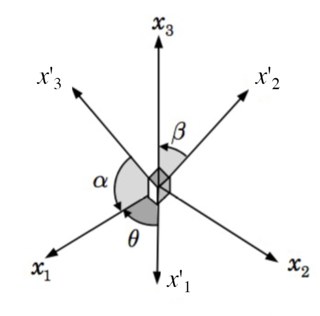
For example, in the figure above:

\[ \alpha_{11} = \cos{\theta} \hspace{0.5cm} \alpha_{31} = \cos{\alpha} \hspace{0.5cm} \alpha_{23} = \cos{\beta} \]

Therefore:

\[\begin{split} \mathbf{v'}= \begin{bmatrix} \cos{\phi} & \sin{\phi} \\ -\sin{\phi} & \cos{\phi} \\ \end{bmatrix} \mathbf{v} \hspace{0.2cm} = \hspace{0.2cm} \begin{bmatrix} \cos{\phi} & \cos{(90 - \phi)} \\ \cos{(90 + \phi)} & \cos{\phi} \\ \end{bmatrix} \mathbf{v} \end{split}\]

Where \(90 - \phi\) is the angle between \(x'_1\) and \(x_2\) and \(90 + \phi\) is the angle between \(x'_2\) and \(x_1\).

A word of caution!

\[ \color{red}{\text{Vector represented in new basis}} \hspace{2.5cm} \mathbf{\color{red}{v'} = \color{purple}{A} \color{blue}{v}} \hspace{2.5cm} \color{blue}{\text{Vector represented in old basis}} \]

\[\begin{split} \color{red}{\mathbf{v'}} = \begin{bmatrix} \color{purple}{\cos{\phi}} & \color{purple}{\sin{\phi}} \\ \color{purple}{-\sin{\phi}} & \color{purple}{\cos{\phi}} \\ \end{bmatrix} \color{blue}{\mathbf{v}} \end{split}\]

\[ \color{purple}{\text{Clockwise rotation by} \hspace{0.1cm} \phi \hspace{1cm} \text{Matrix describing change of basis} \hspace{1cm} \mathbf{New \hspace{0.1cm} basis \hspace{0.1cm} vectors \hspace{0.1cm} are \hspace{0.1cm} ROWS}} \]

\[ \color{red}{\text{New basis vector}} \hspace{2cm} \mathbf{\color{red}{\hat{e}'} = \color{purple}{A^T} \color{blue}{\hat{e}}} \hspace{2cm} \color{blue}{\text{Old basis vector}} \]

\[\begin{split} \color{red}{\mathbf{\hat{e}'}} = \begin{bmatrix} \color{purple}{\cos{\phi}} & \color{purple}{- \sin{\phi}} \\ \color{purple}{\sin{\phi}} & \color{purple}{\cos{\phi}} \\ \end{bmatrix} \color{blue}{\hat{e}} \end{split}\]

\[ \color{purple}{\text{Anticlockwise rotation by} \hspace{0.1cm} \phi \hspace{1cm} \text{Matrix describing basis transformation} \hspace{1cm} \mathbf{New \hspace{0.1cm} basis \hspace{0.1cm} vectors \hspace{0.1cm} are \hspace{0.1cm} COLUMNS}} \]

Vector Calculus

Vector calculus is the field of mathematics that handles differentiation and integration of vector fields.
It allows us to describe the spatial variation in scalar and vector fields.

Vector derivatives

Scalar (e.g time)

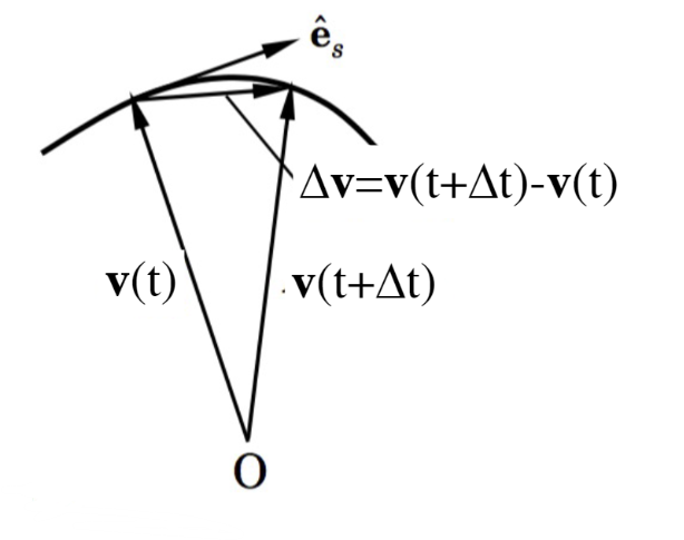
Taking the derivative of a vector gives:

\[\begin{split} {\frac{d\mathbf{v}}{dt} = \begin{pmatrix} \frac{d v_1}{dt} & \frac{d v_2}{dt} & \frac{d v_1}{dt} \\ \end{pmatrix}} \end{split}\]

From first principles, we know:

\[ {\frac{d\mathbf{v}}{dt} = \lim_{\Delta t \to 0} \frac{\mathbf{v}(t + \Delta t) - \mathbf{v}(t)}{\Delta t}} \]

The derivative of the vector usually has a different direction to v.
Remember that

\[ {\mathbf{v} = v_1 \hat{\mathbf{e}}_1 + v_2 \hat{\mathbf{e}}_2 + v_3 \hat{\mathbf{e}}_3} \]

Therefore, taking the derivative gives:

\[ {\frac{d \mathbf{v}}{dt} = \frac{dv_1}{dt} \hat{\mathbf{e}}_1 + \frac{dv_2}{dt} \hat{\mathbf{e}}_2 + \frac{dv_3}{dt} \hat{\mathbf{e}}_3 + \color{blue}{v_1 \frac{d\mathbf{\hat{e}_1}}{dt} + v_2 \frac{d\mathbf{\hat{e}_2}}{dt} + v_3 \frac{d\mathbf{\hat{e}_3}}{dt}}} \]

for Cartesian systems, these terms are = 0

Del Operator

\[\begin{split} {\nabla = \hat{e}_1 \frac{\partial}{\partial x_1} + \hat{e}_2 \frac{\partial}{\partial x_2} + \hat{e}_3 \frac{\partial}{\partial x_3} = \begin{bmatrix} \frac{\partial}{\partial x_1} & \frac{\partial}{\partial x_2} & \frac{\partial}{\partial x_3} \\ \end{bmatrix}} \end{split}\]

The Del operator has some properties of a vector, but not all. Namely, it is not commutative.

\[ {\mathbf{v} \cdot \nabla \phi \neq (\nabla \cdot \mathbf{v}) \phi} \]

Gradient

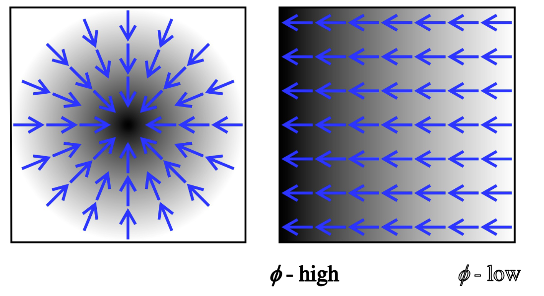
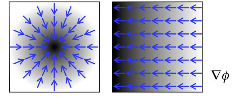
The gradient is a vector measure of change in scalar field with distance. Blue arrows illustrate the gradient for field \(\phi\)

\[ {\nabla \phi = \Biggl(\frac{\partial \phi}{\partial x_1}, \frac{\partial \phi}{\partial x_2}, \frac{\partial \phi}{\partial x_3}\Biggr)} \]

Directional Derivatives: Space

By considering the change in \(\phi\) over a small distance ds, we can deduce that

\[ {d\phi = \frac{\partial \phi}{\partial x_1} ds_1 + \frac{\partial \phi}{\partial x_2} ds_2 + \frac{\partial \phi}{\partial x_3} ds_3} \]

\[\begin{split} {d\phi} = \Biggl( \frac{\partial \phi}{\partial x_1}, \frac{\partial \phi}{\partial x_2}, \frac{\partial \phi}{\partial x_3} \Biggr) \cdot \begin{pmatrix} ds_1 \\ ds_2 \\ ds_3 \\ \end{pmatrix} = \nabla \phi \cdot \mathbf{ds} \end{split}\]

Vector Products with Derivatives

Divergence of a Vector

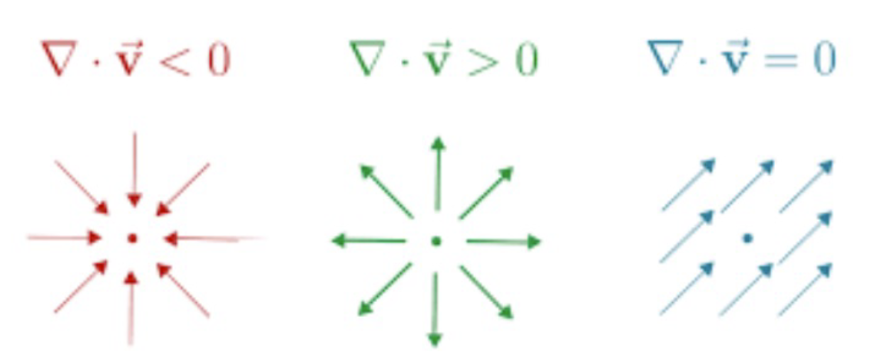
Divergence of a vector field represents the net outward flux per unit volume, i.e the measure of source/sink of flow. It is a scalar quantity.

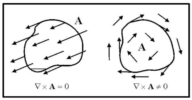
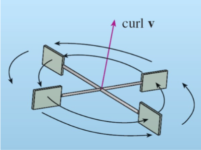
\[ {\nabla} \cdot \mathbf{v} = \sum_{i = 1,3} \frac{\partial v_i}{\partial x_i} = \frac{\partial v_1}{\partial x_1} + \frac{\partial v_2}{\partial x_2} + \frac{\partial v_3}{\partial x_3} \]

Curl of a Vector

The curl of a vector represents the amount of turn or spin (vorticity) in a vector field. This is a vector quantity.

\[\begin{split} {\nabla \times \mathbf{v} = \begin{pmatrix} \frac{\partial v_3}{\partial x_2} - \frac{\partial v_2}{\partial x_3} \\ \frac{\partial v_1}{\partial x_3} - \frac{\partial v_3}{\partial x_1} \\ \frac{\partial v_2}{\partial x_1} - \frac{\partial v_1}{\partial x_2} \\ \end{pmatrix}} \end{split}\]

Useful Calculus Theorems

Take a volume V enclosed by a surface S within a vector field v with continous partial derivatives.
Then the flow perpendicular to the boundary is: \(\;\; \mathbf{v} \cdot \mathbf{\hat{n}} \;\; \) and the flow parallel to the boundary is: \(\;\; \mathbf{v} \cdot \mathbf{\hat{t}} \;\; \).
These can be used to simplify integration over volumes or closed surfaces as well as gain understanding of the meaning of divergence and curl.

Gauss Divergence Theorem

\[ {\int_{V} \nabla \cdot \mathbf{v} d\mathbf{x} = \oint_S \mathbf{v} \cdot \mathbf{\hat{n}} \; ds} \]

Imagine a very small sphere with radius a and boundary S around a point P.

\[ {(\nabla \cdot \mathbf{v})_P \frac{4}{3} \pi a^3 = \oint_{S_a} \mathbf{v} \cdot \mathbf{\hat{n}} \; ds} \]

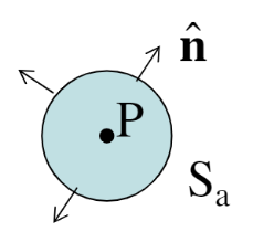
If the volume is taken small enough that the divergence can be considered constant and equal to \((\nabla \cdot \mathbf{v})_P\), then this illustrates that the divergence in this small sphere with volume \(V_a\) corresponds to the net in/outflow of material across its boundary \(S_a\).

Stokes Theorem

\[ {\int_{V} \nabla \times \mathbf{v} d\mathbf{x} = \oint_S \mathbf{v} \cdot \mathbf{\hat{t}} \; ds} \]

The right-hand side of the equation gets larger if the velocities are more parallel to the boundary, or if the vector field is spinning in a consistent direction (i.e there is circulation around the boundary).

Similar to Gauss Theorem, imagine a very small disk with radius a and boundary \(\mathit{C_a}\) around a point P.

\[ {(\nabla \times \mathbf{v})_P \pi a^2 = \oint_{C_a} \mathbf{v} \cdot \mathbf{\hat{t}} \; ds} \]

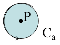
If the disk is taken small enough that the curl of \(\mathbf{v}\) can be considered constant, then this illustrates that the curl in this small disk with area \(S_a\) corresponds to the net rotation of material around its boundary \(C_a\).

Practise

• Try \(\color{blue}{\text{Exercise 5}}\) and \(\color{blue}{\text{Exercise 6}}\) to practise these concepts