1.1 Continuum Mechanics and Vector Calculus#
Lecture 1.1
Saskia Goes, s.goes@imperial.ac.uk
Table of Contents#
Primary Learning Materials#
Lecture notes in ppt or Jupyter notebook
Problem sets and solutions in Jupyter notebook
All content available on GitHub
Recommended reading#
No textbook is required for this module, however the following texts may be helpful
Introduction to Continuum Mechanics, W.M. Lai, D. Rubin, E. Krempl, 4th edition, Elsevier – available in electronic form through IC library
An Introduction to Continuum Mechanics, J.N. Reddy, 2nd edition, Cambridge University Press, 2013
These books use similar notation as this course and cover the mathematical background for first part of this class. Different reading may be suggested for other parts of the course
Introduction#
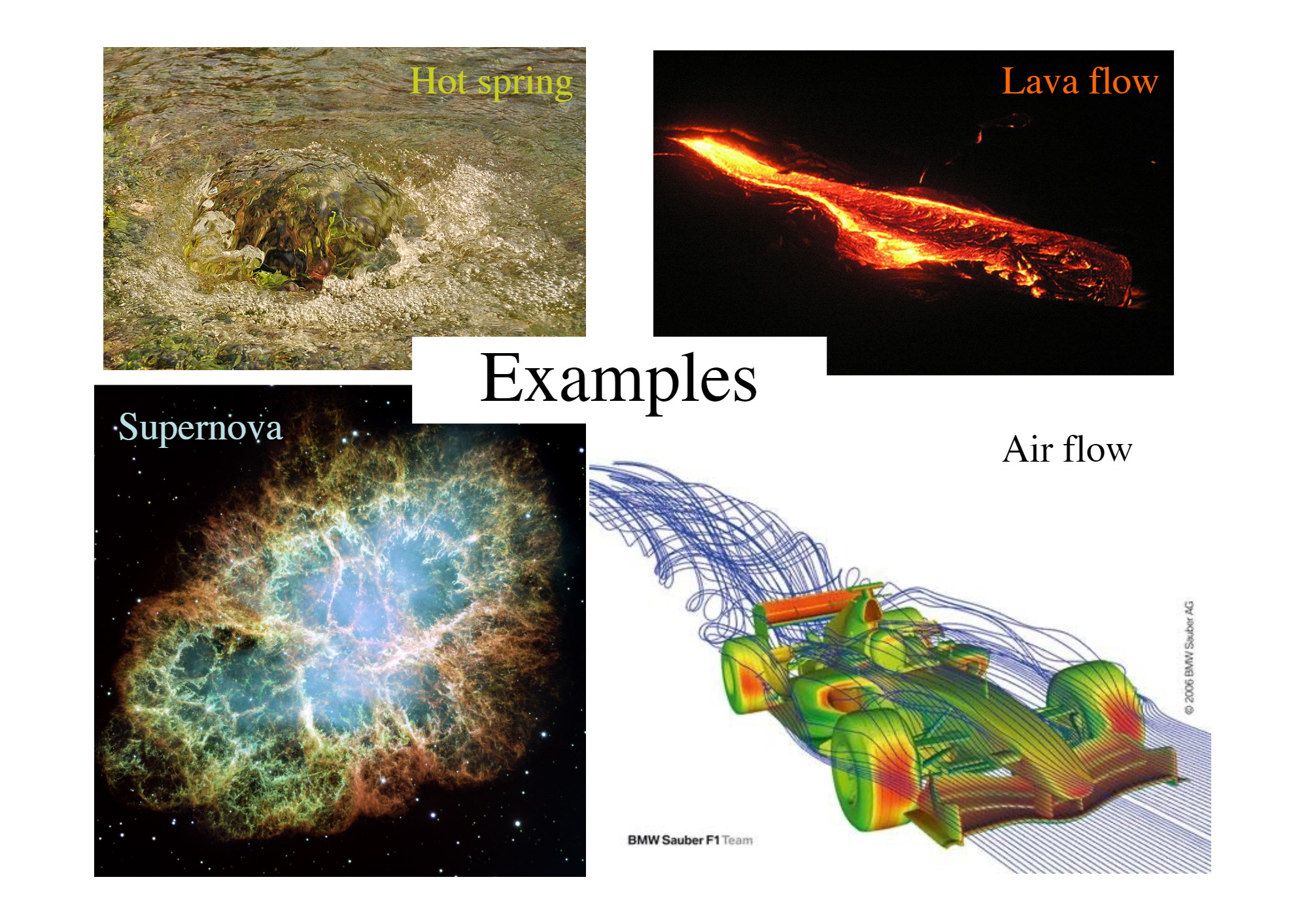
Continuum Mechanics#
Macroscopic description of the collective behaviour of atoms/molecules in the limit where scale of interest >> scale of the individual components
A material, be it solid, liquid, or gas is treated as a hypothetical continuum where all quantities vary continuously so that spatial derivatives exist -In such a treatment, we can consider infinitesimally small volumes of the material and define point quantities, like mass, velocity, stress -Such a description has been found to be applicable in a wide range of problems in engineering and physical sciences
Continuum Mechanics Equations#
General:
Kinematics – describing deformation and velocity without considering forces
Dynamics – equations that describe force balance, conservation of linear and angular momentum
Thermodynamics – relations temperature, heat flux, stress, entropy
Material Specific:
Constitutive equations - relations describing how material properties vary as a function of T,P, stress, etc. Such material properties govern dynamics (e.g. density), response to stress (viscosity, elastic parameters), heat transport (thermal conductivity, diffusivity)
These equations yield a set of Partial Differential Equations that can be solved for displacement, velocity, temperature, etc…
Differential Equations#
Ordinary Differential Equations - describe how variables depend on a single independent parameter (e.g. time or distance). Take Newton’s second law for example,
Partial Differential Equations - describe how variables depend on several independent parameters (e.g. time, x,y,z coordinates). For example, the thermal diffusion equation,
\(\partial\) - partial derivative
Vectors and Tensors#
Revision topics for vectors
Addition, linear independence
Orthonormal Cartesian bases, transformation
Multiplication
Derivatives, del, div, curl
Revision / introductory topics for tensors
Tensors, rank, stress tensor
Index notation, summation convention
Addition, multiplication
Tensor calculus: gradient, divergence, curl, ect…
Learning Outcomes #
Be able to perform vector/tensor operations (addition, multiplication) on Cartesian orthonormal bases
Be able to do basic vector/tensor calculus (time and space derivatives, divergence, curl of a vector field) on these bases.
Perform transformation of a vector from one Cartesian basis to another.
Understand differences/commonalities between tensor and vector
Familiarity with index notation and Einstein convention
Introduction to Vectors and Tensors#
Continuum mechanics equations require vectors and tensors, e.g. velocity is a vector, with magnitude and direction in 3-D, and so are forces like gravity. The components of a vector depend on the coordinate system chosen to represent them in. However, the actual size and orientation of the vector is not dependent on the choice of coordinate system
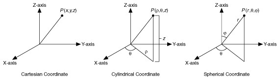
note the size and orientation of the vector is the same regardless of coordinate system
Key Characteristics of a Vector#
Which of the following are true of vectors?
Anything that is not a scalar
Has three components
Has magnitude and direction
Depends on coordinate frame
Velocity and rotation are two examples
Multiplication of two vectors gives another vector
Notation#
Vectors writen as \(\boldsymbol{v}\), \(\bar{v}\), or \(\overrightarrow{v}\)
Length of vectors written as \(v\) or \(\lvert \boldsymbol{v} \rvert\)
Vector in Cartesian components written as \(v_x , v_y , v_z\)
Index notation, \(v_i\) where \(i = x,y,z\) or \(i = 1,2,3\)
Unit vector along direction of \(\boldsymbol{v}\) written as \(\hat{e_v}\)
The unit vector is defined as follows,
Hence,
Vector properties#
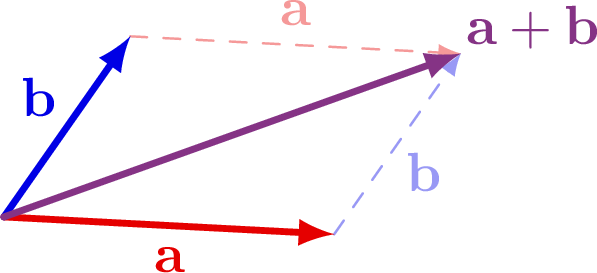
Vectors satisfy certain rules of addition and scalar multiplication
\(\mathbf{a} + \mathbf{b} = \mathbf{b} +\mathbf{a}\) (commutative)
\((\mathbf{a} + \mathbf{b}) + \mathbf{c} = \mathbf{a} +(\mathbf{b} + \mathbf{c})\) (associative)
\(\alpha (\mathbf{a} + \mathbf{b}) = \alpha\mathbf{a} + \alpha\mathbf{b}\) (distributive)
\(\mathbf{a} + 0 = \mathbf{a}\) (zero vector)
\(1 \cdot{} \mathbf{a} = \mathbf{a} \cdot 1\) and \(0 \cdot{} \mathbf{a} = 0\)
We will see that similar rules apply to tensors. See http://mathworld.wolfram.com/Vector.html for more details
Finite rotation “Vector”#
A finite rotation can be represented as a pseudo-vector. The direction of the vector forms the axis of rotation and the magnitude represents the angle rotated. For the direction of rotation the right hand rule is used where the thumb aligns to the axis of rotation and the fingers point in the direction of rotation.
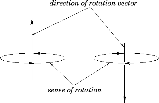
The reason that finite rotation is a pseudo-vector is that the addition of two finite rotations is not commutative. Hence finite rotations do not satisfy the properties of a vector. However, an infinitesimal rotation is considered a vector.
Linear independence#
Vectors \(\mathbf{v_1}\) through \(\mathbf{v_n}\) are linearly dependent if coefficients \(c_i\) can be found such that:
\(c_1 \mathbf{v_1} + c_2 \mathbf{v_2} + c_3 \mathbf{v_3} + ... + c_n \mathbf{v_n} = 0\) where \(c_i \neq 0\)
Hence, vectors are linearly independent if they cannot be written as linear combinations of each other.
Two linearly dependent vectors are parallel/colinear
Three linearly dependent vectors are coplanar
Four or more vectors are always linearly dependent
Important for defining bases and finding independent solutions to a problem. Practice for this is in Exercise 2
Inner, dot, or scalar product#
Produces a scalar (hence the name scalar product)
gives the projection of \(\mathbf{F}\) on \(\mathbf{d}\) scaled by \(\lvert \mathbf{d} \rvert\)
\(\mathbf{F} \cdot \mathbf{d} = \mathbf{d} \cdot \mathbf{F}\)
\(\mathbf{a} \cdot \mathbf{a} = length(\mathbf{a})^2 = \lvert \mathbf{a} \rvert^2\)

The scalar product has several physical interpretations. For example, if \(\mathbf{F}\) is force and \(\mathbf{d}\) is displacement, then \(\mathbf{F} \cdot \mathbf{d}\) is the work done by the force \(\mathbf{F}\) for displacement \(\mathbf{d}\)
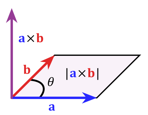
Cross, vector, or outer product#
Produces a vector
Magnitude of cross product is the area of a parallellogram spanned by \(\mathbf{a}\) and \(\mathbf{b}\)
Direction of cross product is normal to the plane of \(\mathbf{a}\) and \(\mathbf{b}\)
if \(\mathbf{a}\) and \(\mathbf{b}\) are parallel cross product = 0
\(\mathbf{a} \times \mathbf{b} = -\mathbf{a} \times \mathbf{b}\)
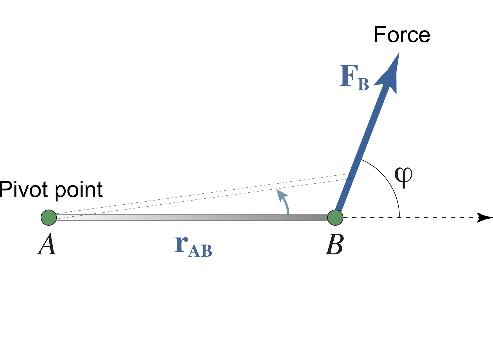
One physical application of the cross product is in calculating moments. If \(\mathbf{r_{AB}}\) is the moment arm between the pivot point A and the force \(\mathbf{F_B}\), then the resulting moment is calculated as
Product calculations#
The products of vectors in rectangular Cartesian coordinates:
2D
3D
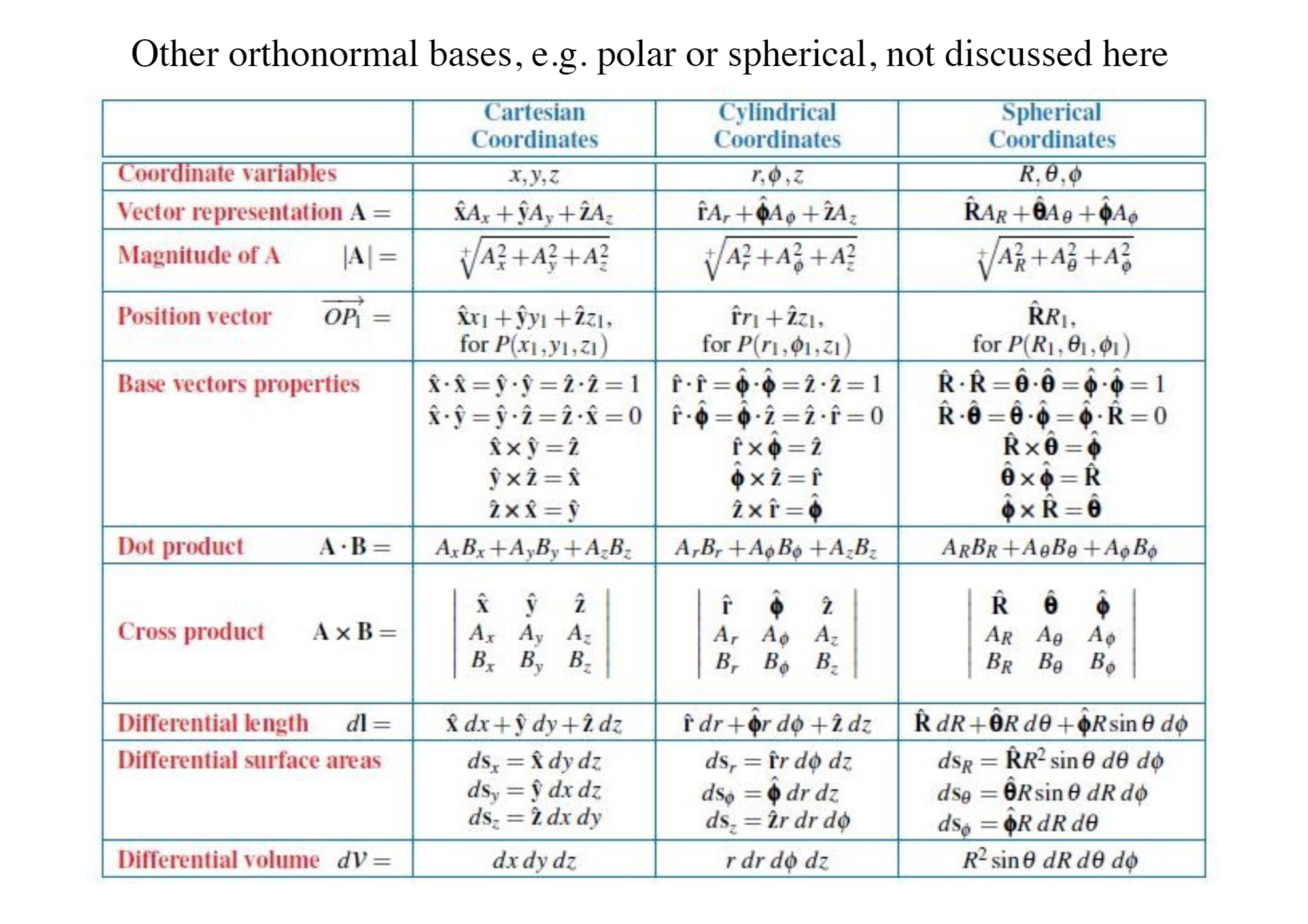
Rectangular Cartesian Coordinate System#
The rectangular Cartesian coordinate system has an orthonormal basis. This means that the basis vectors are all unit vectors, orthogonal to each other.
Cartesian orthonormal bases will be assumed for most of this class
Equivalence of Cartesian geometric and algebraic dot product#
Cartesian algebraic cross product#
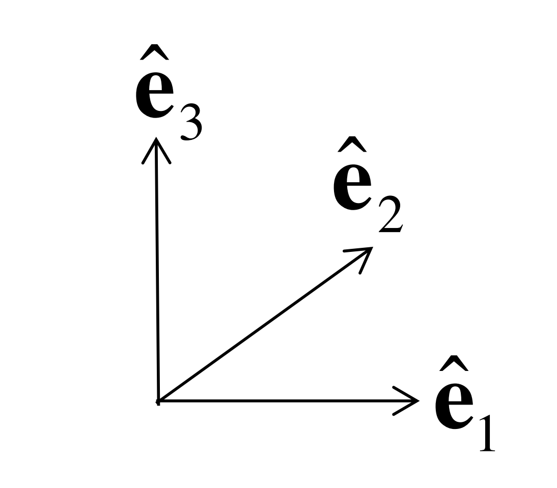
Recall that the result of the cross product has a magnitude equal to the area of a parallellogram formed by the two vectors, and has direction normal to the parallellogram. From this it can be seen that \(\hat{\mathbf{e_1}} \times \hat{\mathbf{e_2}} = \hat{\mathbf{e_3}}\). Using the properties of cross product we can also see that \(\hat{\mathbf{e_2}} \times \hat{\mathbf{e_1}} = -\hat{\mathbf{e_3}}\)
Using the basis vectors, the 2D cross product result can be shown fully as:
Triple Products #
\(\mathbf{a}(\mathbf{b}\cdot\mathbf{c})\) is a vector multiplied by a scalar
\(\mathbf{a}\cdot(\mathbf{b}\times\mathbf{c})\) is the scalar triple product
\(\mathbf{a}\cdot(\mathbf{b}\times\mathbf{c}) =(\mathbf{a}\times\mathbf{b})\cdot\mathbf{c}\)
\(\mathbf{a}\cdot(\mathbf{b}\times\mathbf{c}) = \mathbf{c}\cdot(\mathbf{a}\times\mathbf{b}) = \mathbf{b}\cdot(\mathbf{c}\times\mathbf{a})\) (with cyclical permutation)
\(\mathbf{a}\cdot(\mathbf{b}\times\mathbf{c}) = -\mathbf{a}\cdot(\mathbf{c}\times\mathbf{b}) =-\mathbf{c}\cdot(\mathbf{b}\times\mathbf{a}) = -\mathbf{b}\cdot(\mathbf{a}\times\mathbf{c})\) (with order changed)
\(\mathbf{a}\cdot(\mathbf{b}\times\mathbf{c}) = 0 \) if \(\mathbf{a}, \mathbf{b}, \mathbf{c}\) are coplanar
\(\mathbf{a} \times (\mathbf{b} \times \mathbf{c})\) lies in plance formed by \(\mathbf{b} \times \mathbf{c}\) normal to \(\mathbf{a}\)
\( \neq (\mathbf{a} \times \mathbf{b}) \times \mathbf{c}\)
\( = (\mathbf{a} \cdot \mathbf{c}) \mathbf{b} - (\mathbf{a} \cdot \mathbf{b}) \mathbf{c}\)
Covered so far#
Revision of main characteristics of a vector
Linear independence of vectors
Vector products: dot product, cross product
Definition Cartesian orthonormal basis
Take a break, then try yourself#
If the material covered so far was all familiar, please skip to \(\color{blue}{\text{Exercise 2}}\) in the notebook
If you would benefit from recapping vector products, please look at \(\color{green}{\text{Exercise 1}}\) first