7.1 Solving Navier-Stokes Numerically#
Lecture 7.1
Stephen Neethling
Table of Contents#
Outline#
Discuss some of the relevant features of the Navier-Stokes equation
Derive and discuss the fully implicit solution to the NS equation
Discuss a semi-implicit method for solving the equation (Pressure projection method)
Implement the pressure projection method
Demonstrate and discuss the solution of some example problems
Learning Objectives#
Derive an implicit discretisation for the NS equation
Derive a pressure projection discretisation for solving the NS equation
Derive appropriate boundary conditions for the problem
Learn how to implement a solver for the Pressure Poisson problem
Learn how to implement an explicit solver for the momentum equation, including the appropriate use of up-winding
Combine the solvers into a single Navier-Stokes solver capable of solving a range of fluid flow problems
# Import packages for notebook here
import numpy as np
import matplotlib.pyplot as plt

%matplotlib inline
Method 1: Implicit Matrix Solution for all Variables#
One way to achieve continuity is to simultaneously solve for the velocity and pressure values
Using a Crank-Nicolson implicit scheme (2nd order accurate in time)
Crank-Nicolson carries out the spatial derivatives using an average of the current and future time step
\(\mathbf{K, C}\) and \(\mathbf{C^T}\) are the matrices for the discretisation of the viscosity (Laplacian), gradient operator and divergence respectively
\(\mathbf{A(\tilde{u})}\) is the matrix containing the discretisation for the momentum advection term.
Note that the matrix for the momentum advection term depends on the velocity. This is what make the problem non-linear
The equations on the previous slide can be rearranged into a single matrix where the velocities and pressures at the next time step are a function of the current velocities:
The next decision is the choice use for the velocity in the momentum advection term
The easiest, but least accurate is to use the velocity from the current time step, \(\mathbf{u}^n\)
More accurate would be to use the same average as used in the rest of the Crank-Nicolson scheme, \(\frac{1}{2}(\mathbf{u}^{n+1} + \mathbf{u}^n)\). This is more accurate, by the problem is that it requires iteration and multiple assembly and solves of the matrix
The big problem with this method is that it is computationally expensive because the matrix to be solved is large and difficult to solve because
Method 2: Split the Pressure and Velocity Solves#
Firstly, we need an equation for the pressure solve
We can achieve this by taking the divergence of the momentum equations:
This can be simplified using the fact that the divergence of the Laplacian of the velocity and the divergence of the rate of change of velocity are both commutable and therefore zero given continuity:
Pressure Poisson Equation#
This results in the following equation:
This is known as the pressure Poisson equation. It is very similar to the Laplace equation we solved in the previous lecture, except that it has a non-zero RHS
This equation is therefore quite easy to solve and generally well behaved in terms of its convergence
In 2D this can be further simplified and expanded to:
Finite Difference approximation of Pressure Poisson Equation#
We can do a finite difference approximation of the this equation
I will assume that \(\Delta x = \Delta y\)
We could now simply use an explicit calculation of the new velocities using a discretisation of the momentum equation together with the current velocity and pressure equations and then use the new velocities to calculate the new pressures
Would work for a while, but numerical errors will mean that continuity violations will grow with time
Pressure Projection#
In this method we will calculate an intermediate velocity and then use this velocity to calculate the pressure gradient required to make the velocity at the next step divergence free
Start by calculating a velocity \( \mathbf{u^* } \) that ignores the contribution from the pressure gradient (note that this is an explicit forward Euler approximation):
From the full equation we therefore know that:
If we take the divergence of both sides:
What we are trying to enforce is that the final velocity is divergence free \(( \nabla \cdot \mathbf{u}^{n+1} = 0 )\)
We therefore have the following calculation sequence:
Calculate the intermediate velocity explicitly:
Calculate the pressure implicitly using the following pressure Poisson equation (remember to impose any pressure boundary conditions):
Calculate the velocity at the new time step (also remember to impose any velocity boundary conditions):
Pressure Projection- Finite Difference (2D)#
Viscous term:
Momentum advection term:
Note that we need to use upwind discretisations of velocity to be stable at high Reynolds numbers
Laplacian of the Pressure:
Gradient of the Pressure:
Divergence of the intermediate velocity:
Centeral difference
Upwind
Central difference is more accurate, but can cause problems especially at very high Reynolds numbers
Upwinding is less accurate, but is more stable
I will generally use central difference approximations for the RHS of the pressure Poisson equation
Solid Boundaries in Fluid Dynamics#
No Slip Boundary Condition
A useful assumption for most solid boundaries
Together with no flux through the boundary this implies a zero velocity vector at the boundary
Not completely true at the very smallest scales
Some molecular slip may need to be included for micro or nano scale fluid flows
Good approximation for macroscopic flows
We will be using no slip conditions in all the examples in this lecture
Velocity Boundary Layers
Some flows will have velocity boundary layers against solid walls
No slip at the wall, but rapid increase towards free stream velocity away from the wall
Boundary layers often thin compared to the scale of the system
Especially true for turbulent flows
Can also occur in entry regions for laminar flows
More on turbulent flow in the next lecture
Modelling Systems with Boundary Layers
Could simply have enough resolution near the wall to resolve the wall
Can be computationally very expensive especially in large scale simulations
Simplest approximation is that there is full slip at the boundary
Not a bad approximation in very turbulent flows, but implies that there are no shear stresses on the wall
Can use a sub-resolution model to impose a stress at the boundary that is a function of the velocity at the boundary
More complex models will include predictions for the velocity profile in this boundary region and a more complex inter-relationship between the stress at the wall and the velocity profile in the resolved near wall region
Pressure Condition at No-Slip Boundary#
To solve the system we need boundary conditions for the pressure and the velocity
Lets consider a vertical wall and the momentum balance in the direction normal to the wall:
This says that the total normal stress at the boundary should be zero. For no slip boundaries the shear stress component into the boundary will be small (or zero for fully developed flows)
The most commonly used pressure boundaries for these walls is thus:
The Code (with explicit loops)#
I am firstly going to show the code with explicit loops and if statements
Hopefully make what is being done easier to understand
This is exactly how I would code this in a compiled language like C/C++
Unfortunately Python is an interpreted language and very inefficient in its implementation of for loops and conditions
Vectorised portions of the code are executed using libraries written in C++ and so are fast
Calculating the Intermediate Velocities#
def calculate_intermediate_velocity(nu, u, v, u_old, v_old, dt, dx, dy):
""" Calculate the intermediate velocities.
"""
imax = len(u)
jmax = np.size(u)//imax
for i in range(1,imax-1,1):
for j in range(1,jmax-1,1):
#viscous (diffusive) term first
u[i,j] = u_old[i,j] + dt * nu * ((u_old[i+1,j]+u_old[i-1,j]-2.*u_old[i,j])/(dx**2)
+(u_old[i,j+1]+u_old[i,j-1]-2.*u_old[i,j])/(dy**2))
v[i,j] = v_old[i,j] + dt * nu * ((v_old[i+1,j]+v_old[i-1,j]-2.*v_old[i,j])/(dx**2)
+(v_old[i,j+1]+v_old[i,j-1]-2.*v_old[i,j])/(dy**2))
#add the momentum advection terms using upwinding
if (u_old[i,j]>0.0):
u[i,j] -= dt*(u_old[i,j]*(u_old[i,j]-u_old[i-1,j])/dx)
v[i,j] -= dt*(u_old[i,j]*(v_old[i,j]-v_old[i-1,j])/dx)
else:
u[i,j] -= dt*(u_old[i,j]*(u_old[i+1,j]-u_old[i,j])/dx)
v[i,j] -= dt*(u_old[i,j]*(v_old[i+1,j]-v_old[i,j])/dx)
if (v_old[i,j]>0.0):
u[i,j] -= dt*(v_old[i,j]*(u_old[i,j]-u_old[i,j-1])/dx)
v[i,j] -= dt*(v_old[i,j]*(v_old[i,j]-v_old[i,j-1])/dx)
else:
u[i,j] -= dt*(v_old[i,j]*(u_old[i,j+1]-u_old[i,j])/dx)
v[i,j] -= dt*(v_old[i,j]*(v_old[i,j+1]-v_old[i,j])/dx)
return u, v
  Cell In[2], line 2
    """ Calculate the intermediate velocities.
    ^
IndentationError: expected an indented block
Setting up and Solving the Pressure Poisson Equation#
def calculate_ppm_RHS(rho, u, v, dt, dx, dy):
""" Calculate the RHS of the
Poisson equation resulting from the projection method.
Use central differences for the first derivatives of u and v.
"""
imax = len(p)
jmax = np.size(p)//imax
RHS = np.zeros_like(X)
for i in range(1,imax-1,1):
for j in range(1,jmax-1,1):
RHS[i, j] = rho * ((1.0/dt) * ( (u[i+1, j] - u[i-1, j]) / (2*dx) + (v[i, j+1] - v[i, j-1]) / (2*dy)))
return RHS
def pressure_poisson_jacobi(p, dx, dy, RHS, rtol = 1.e-5, logs = False):
"" Solve the pressure Poisson equation (PPE)
using Jacobi iteration assuming mesh spacing of
dx and dy (we assume at the moment that dx=dy)
and the RHS function given by RHS.
Assumes imposition of a Neumann BC on all boundaries.
Return the pressure field.
""
# our code below is only currently for the case dx=dy
assert dx==dy
# iterate
tol = 10.*rtol
it = 0
p_old = np.copy(p)
imax = len(p)

jmax = np.size(p)//imax
while tol > rtol:
it += 1
for i in range(1,imax-1,1):
for j in range(1,jmax-1,1):
p[i, j] = 0.25*(p_old[i+1, j] + p_old[i-1, j] + p_old[i, j+1] + p_old[i,j-1] - (dx**2)*RHS[i, j])
# apply zero pressure gradient Neumann boundary conditions
for i in range(imax):
p[i,0] = p[i,1]
p[i,jmax-1] = p[i,jmax-2]
for j in range(jmax):
p[0,j] = p[1,j]
p[imax-1,j] = p[imax-2,j]
# fix pressure level - choose an arbitrary node to set p to
# be zero, avoid the corners and set it to an interior location
p[1,1] = 0
# relative change in pressure
tol = sl.norm(p - p_old)/np.maximum(1.0e-10,sl.norm(p))
#swap arrays without copying the data
temp = p_old
p_old = p
p = temp
if logs: print('pressure solve iterations = {:4d}'.format(it))
return p
'def calculate_ppm_RHS(rho, u, v, dt, dx, dy):\n"" Calculate the RHS of the\nPoisson equation resulting from the projection method.\nUse central differences for the first derivatives of u and v.\n""\nimax = len(p)\njmax = np.size(p)//imax\nRHS = np.zeros_like(X)\nfor i in range(1,imax-1,1):\nfor j in range(1,jmax-1,1):\nRHS[i, j] = rho * ((1.0/dt) * ( (u[i+1, j] - u[i-1, j]) / (2*dx) + (v[i, j+1] - v[i, j-1]) / (2*dy)))\nreturn RHS\ndef pressure_poisson_jacobi(p, dx, dy, RHS, rtol = 1.e-5, logs = False):\n"" Solve the pressure Poisson equation (PPE)\nusing Jacobi iteration assuming mesh spacing of\ndx and dy (we assume at the moment that dx=dy)\nand the RHS function given by RHS.\nAssumes imposition of a Neumann BC on all boundaries.\nReturn the pressure field.\n""\n# our code below is only currently for the case dx=dy\nassert dx==dy\n# iterate\ntol = 10.*rtol\nit = 0\np_old = np.copy(p)\nimax = len(p)\n\njmax = np.size(p)//imax\nwhile tol > rtol:\nit += 1\nfor i in range(1,imax-1,1):\nfor j in range(1,jmax-1,1):\np[i, j] = 0.25*(p_old[i+1, j] + p_old[i-1, j] + p_old[i, j+1] + p_old[i,j-1] - (dx**2)*RHS[i, j])\n# apply zero pressure gradient Neumann boundary conditions\nfor i in range(imax):\np[i,0] = p[i,1]\np[i,jmax-1] = p[i,jmax-2]\nfor j in range(jmax):\np[0,j] = p[1,j]\np[imax-1,j] = p[imax-2,j]\n# fix pressure level - choose an arbitrary node to set p to\n# be zero, avoid the corners and set it to an interior location\np[1,1] = 0\n# relative change in pressure\ntol = sl.norm(p - p_old)/np.maximum(1.0e-10,sl.norm(p))\n#swap arrays without copying the data\ntemp = p_old\np_old = p\np = temp\nif logs: print(\'pressure solve iterations = {:4d}\'.format(it))\nreturn p\n'
Calculate Updated Velocity using Pressure Gradient#
def project_velocity(rho, u, v, dt, dx, dy, p):
""" Update the velocity to be divergence free using the pressure.
"""
imax = len(p)
jmax = np.size(p)//imax
for i in range(1,imax-1,1):
for j in range(1,jmax-1,1):
u[i, j] = u[i, j] - dt * (1./rho) * (
(p[i+1, j] - p[i-1, j])/(2*dx) )
v[i, j] = v[i, j] - dt * (1./rho) * (
(p[i, j+1] - p[i, j-1])/(2*dy) )
return u, v
Combine the Previous Functions to solve NS#
def solve_NS(u, v, p, rho, nu, dt, t_end, dx, dy, rtol = 1.e-5, logs = False):
""" Solve the incompressible Navier-Stokes equations
using a lot of the numerical choices and approaches we've seen
earlier in this lecture.
"""
t = 0
u_old = u.copy()
v_old = v.copy()
while t < t_end:
t += dt
if logs: print('\nTime = {:.8f}'.format(t))
# calculate intermediate velocities
u, v = calculate_intermediate_velocity(nu, u, v, u_old, v_old, dt, dx, dy)
# PPM
# calculate RHS for the pressure Poisson problem
p_RHS = calculate_ppm_RHS(rho, u, v, dt, dx, dy)
# compute pressure - note that we use the previous p as an initial guess to the solution
p = pressure_poisson_jacobi(p, dx, dy, p_RHS, 1.e-5, logs)
# project velocity
u, v = project_velocity(rho, u, v, dt, dx, dy, p)
if logs:
print('norm(u) = {0:.8f}, norm(v) = {1:.8f}'.format(sl.norm(u),sl.norm(v)))
print('Courant number: {0:.8f}'.format(np.max(np.sqrt(u**2+v**2)) * dt / dx ))
# relative change in u and v

tolu = sl.norm(u - u_old)/np.maximum(1.0e-10,sl.norm(u))
tolv = sl.norm(v - v_old)/np.maximum(1.0e-10,sl.norm(v))
if tolu < rtol and tolv < rtol: break
#swap pointers without copying data
temp = u_old
u_old = u
u = temp
temp = v_old
v_old = v
v = temp
return u, v, p
Test Example#
Going to solve the code for the specific case of a lid driven cavity
No inflow or outflow
Top boundary has an applied velocity of 1
No slip w.r.t. this movement
All other boundaries are stationary with no slip
Box of size 1x1
This gives a Reynold’s number based on the lid velocity of 10
Note on the Pressure Calculation#
In problems such as this where all the pressure boundaries are Neumann boundaries (gradient boundaries) there is a potential issue with the pressure calculations:
Flow only depends on the gradient of the pressure and therefore adding a constant to all the pressure values does not change the solution
System is under-specified by one degree of freedom
A naïve iteration can therefore drift and never converge
A solution to this problem is to set pressure at one point in the system
For more direct matrix solution methods for systems like this the removal of what is known as the nullspace is required
Call the Function to Solve Lid Driven Cavity#
# physical parameters
rho = 1
nu = 1./10.
# define spatial mesh
# Size of rectangular domain
Lx = 1
Ly = Lx
# Number of grid points in each direction, including boundary nodes
Nx = 51
Ny = Nx
# hence the mesh spacing
dx = Lx/(Nx-1)
dy = Ly/(Ny-1)
# read the docs to see the ordering that mgrid gives us
X, Y = np.mgrid[0:Nx:1, 0:Ny:1]
X = dx*X
Y = dy*Y
# the following is an alternative to the three lines above
#X, Y = np.mgrid[0: Lx + 1e-10: dx, 0: Ly + 1e-10: dy]
# but without the need to add a "small" increment to ensure
# the Lx and Ly end points are included
# time stepping parameters
dt = 2.e-4
t_end = 2.0

# initialise independent variables
u = np.zeros_like(X)
v = np.zeros_like(X)
p = np.zeros_like(X)
# Apply Dirichlet BCs to u and v - the code below doesn't touch
# these so we can do this once outside the time loop
u[:, -1]=1 # set velocity on cavity lid equal to 1
u[:, 0]=0
u[0, :]=0
u[-1, :]=0
v[:, -1]=0
v[:, 0]=0
v[0, :]=0
v[-1, :]=0
import time
start = time.time()
u, v, p = solve_IN(u, v, p, rho, nu, dt, t_end, dx, dy, rtol=1.e-6, logs = True)
end = time.time()
print('Time taken by calculation = ', end - start)
'\n# physical parameters\nrho = 1\nnu = 1./10.\n# define spatial mesh\n# Size of rectangular domain\nLx = 1\nLy = Lx\n# Number of grid points in each direction, including boundary nodes\nNx = 51\nNy = Nx\n# hence the mesh spacing\ndx = Lx/(Nx-1)\ndy = Ly/(Ny-1)\n# read the docs to see the ordering that mgrid gives us\nX, Y = np.mgrid[0:Nx:1, 0:Ny:1]\nX = dx*X\nY = dy*Y\n# the following is an alternative to the three lines above\n#X, Y = np.mgrid[0: Lx + 1e-10: dx, 0: Ly + 1e-10: dy]\n# but without the need to add a "small" increment to ensure\n# the Lx and Ly end points are included\n# time stepping parameters\ndt = 2.e-4\nt_end = 2.0\n\n# initialise independent variables\nu = np.zeros_like(X)\nv = np.zeros_like(X)\np = np.zeros_like(X)\n# Apply Dirichlet BCs to u and v - the code below doesn\'t touch\n# these so we can do this once outside the time loop\nu[:, -1]=1 # set velocity on cavity lid equal to 1\nu[:, 0]=0\nu[0, :]=0\nu[-1, :]=0\nv[:, -1]=0\nv[:, 0]=0\nv[0, :]=0\nv[-1, :]=0\nimport time\nstart = time.time()\nu, v, p = solve_IN(u, v, p, rho, nu, dt, t_end, dx, dy, rtol=1.e-6, logs = True)\nend = time.time()\nprint(\'Time taken by calculation = \', end - start)\n'
Solution for Re = 10#
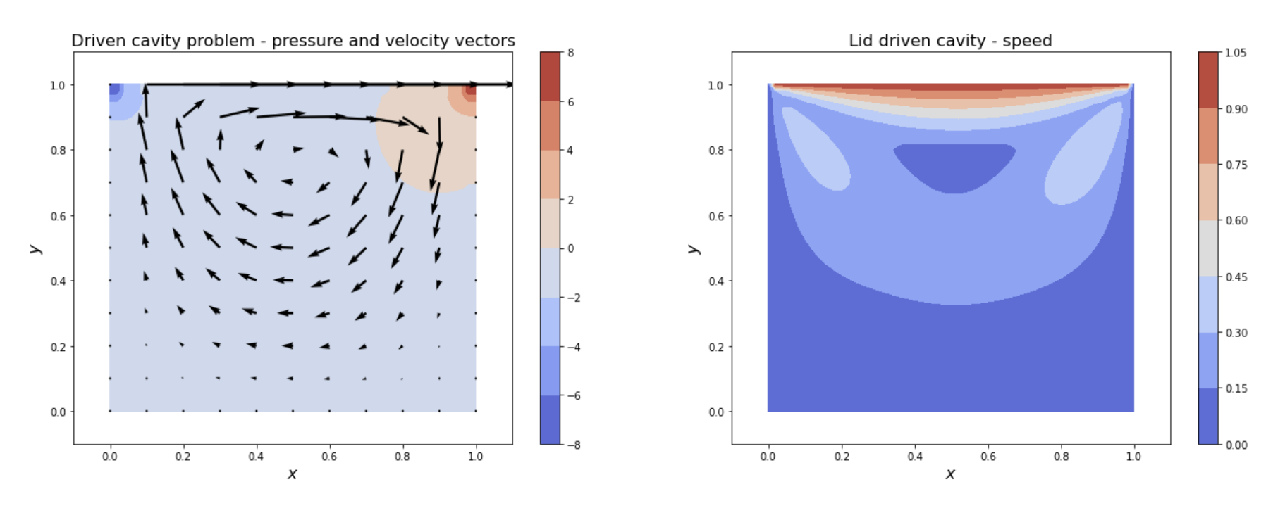
Comparison to High Resolution Simulations for Re = 10#
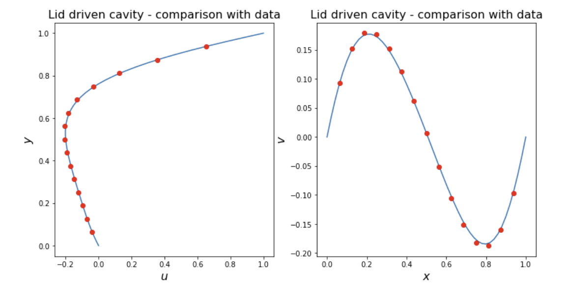
Benchmark date: MARCHI, Carlos Henrique; SUERO, Roberta and ARAKI, Luciano Kiyoshi. The lid-driven square cavity flow: numerical solution with a 1024 x 1024 grid. J. Braz. Soc. Mech. Sci. & Eng. 2009, vol.31, n.3, pp.186-198. http://dx.doi.org/10.1590/S1678-58782009000300004.
Solution for Re = 100#
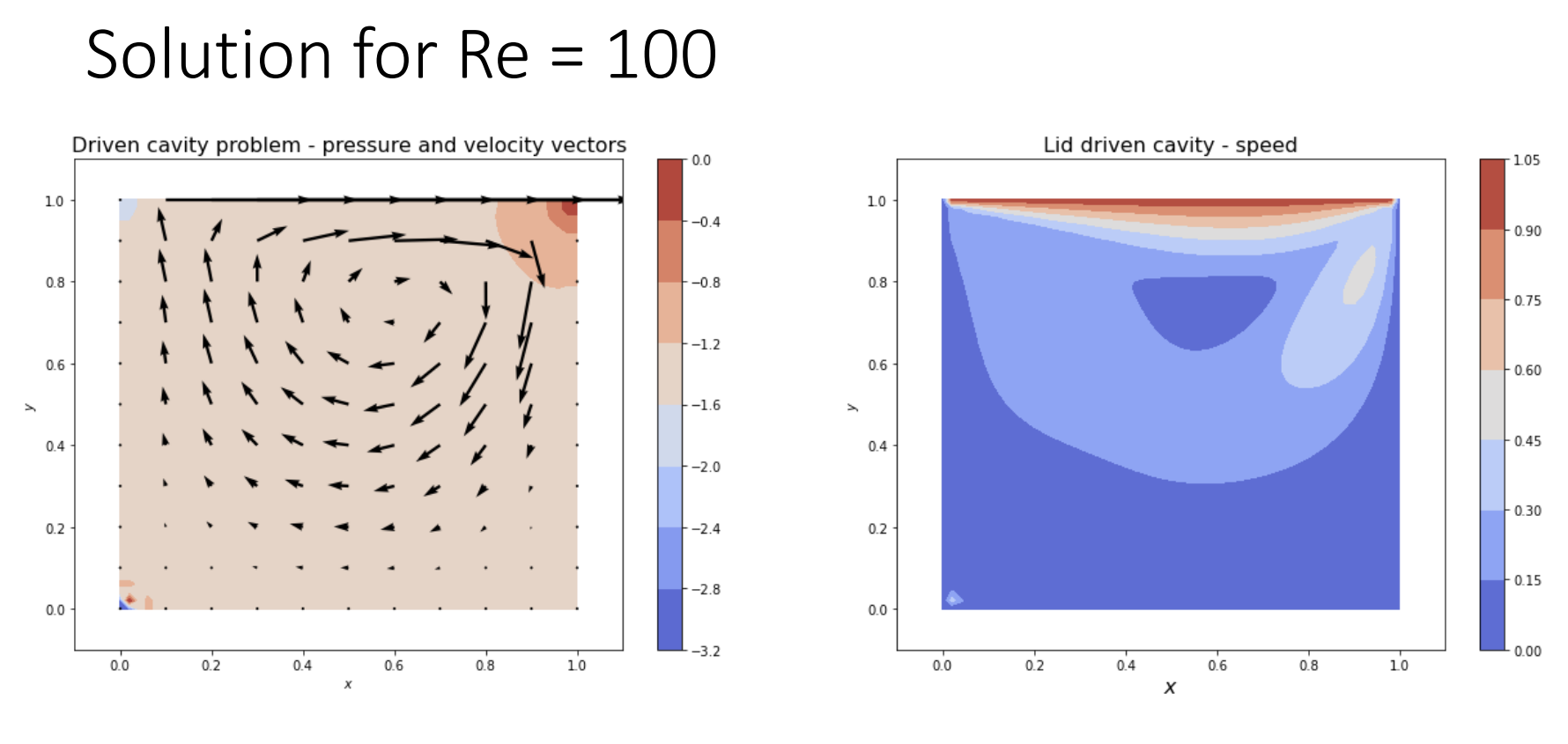
Comparison to High Resolution Simulations for Re = 100#
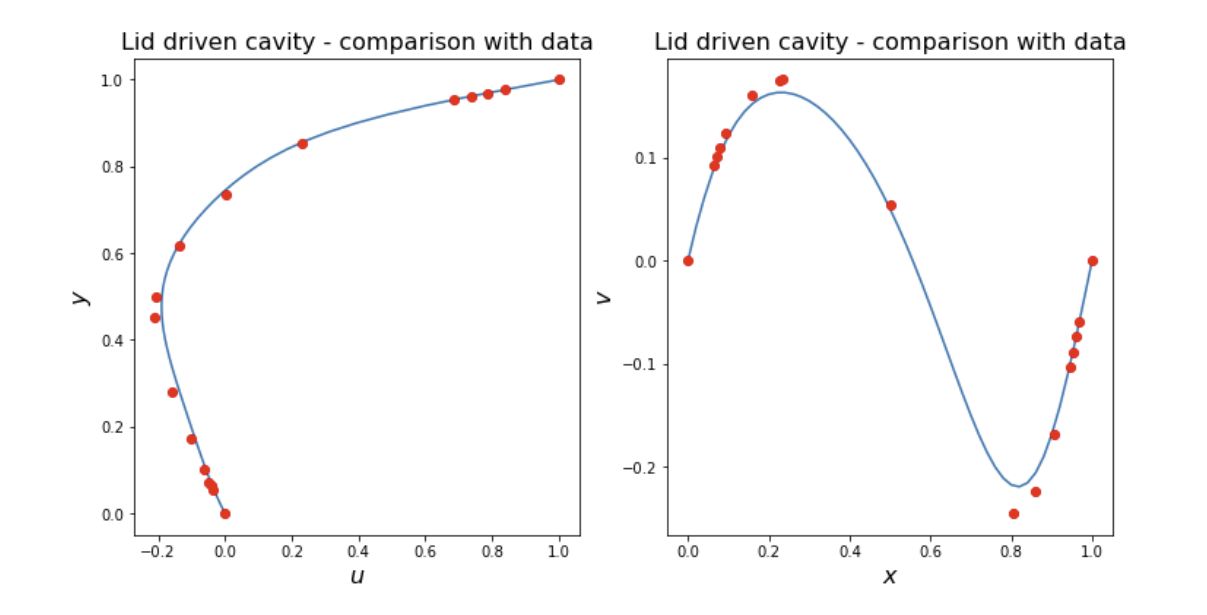
Benchmark date: Ghia, U., Ghia, K. N. & Shin, C. T. High-Re solutions for incompressible flow using the Navier-Stokes equations and a multigrid method. J. Comput. Phys. 48, 387–411 (1982).
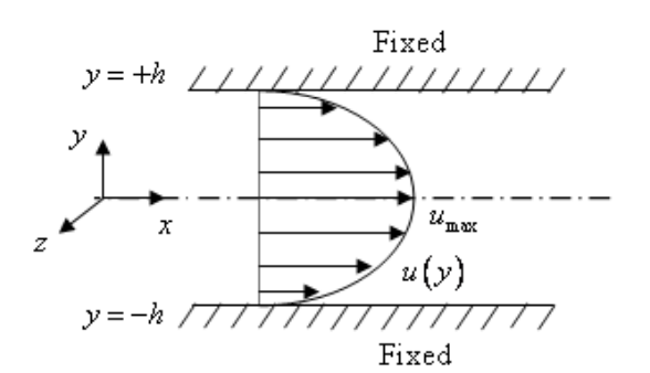
Pressure Driven Steady Flow between Parallel Plates#
An analytical solution for steady state can be derived easily either from the Navier-Stoke equation or by considering a force balance on a unit of fluid:
No time dependency
Only non-zero velocity components are in the x direction
Ignore body forces
Integrate and note that \(u_x = 0\) at \(y = h\) and \(y = -h\):
Pressure Boundary Conditions#
Pressure boundary for the pressure itself is a Dirichlet boundary in
which the pressure is set at the boundary
Note that as a pressure is being specified, there is no issue with drift in pressure and so no arbitrary pressure values need to be set
For the velocity, the easiest boundary to impose is to assume that the fluid flow through the boundary is in the normal direction to boundary
This implies that the velocity components in the other direction/s are zero
This therefore also implies that for an incompressible the gradient in the velocity normal to the boundary is zero
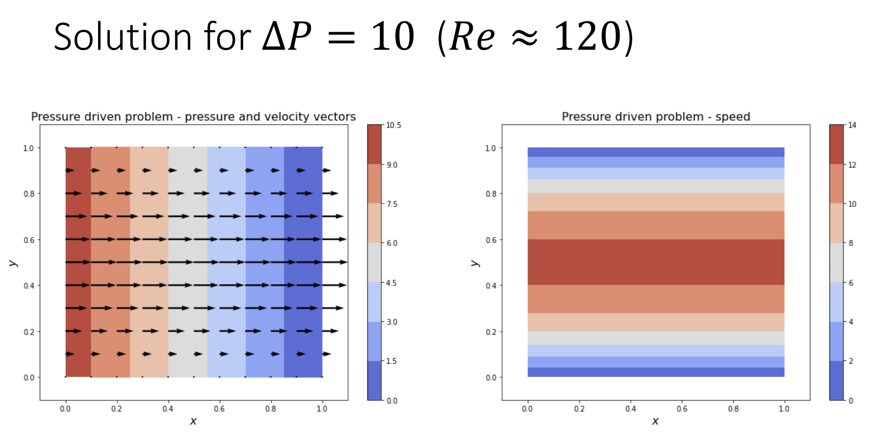
Solution for \(\Delta P = 10 ( Re \approx 120) \)#
Comparison to Theory for \(\Delta P = 10 ( Re \approx 120) \)#
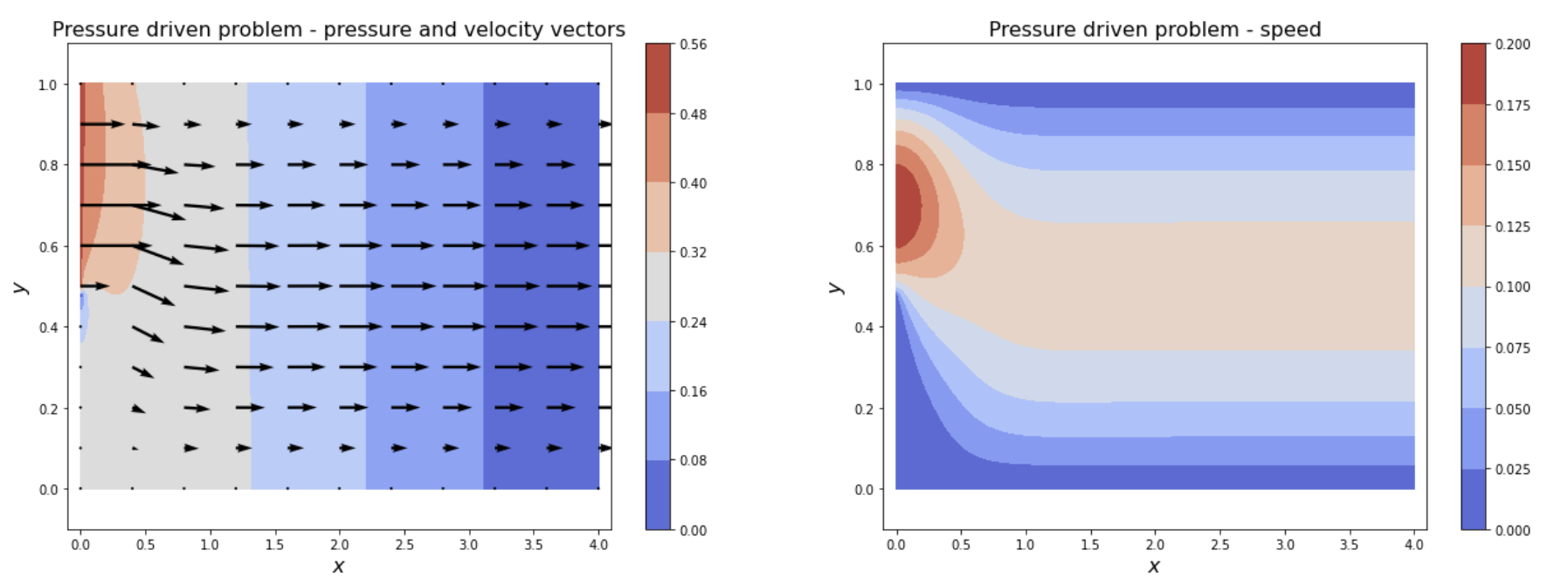
Non-uniform Addition \(\Delta P = 0.5\)#
To make the solution more interesting I have made half the inlet a solid wall and half a pressure boundary
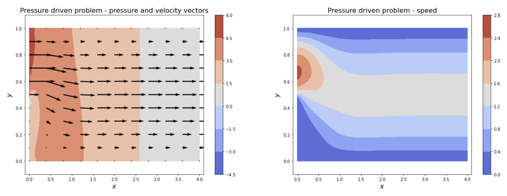
Non-uniform Addition \(\Delta P = 5\)#
Staggered Pressure and Velocity Grid#
-The scheme introduced in this lecture is a widely used basis for carrying out Navier-Stokes simulations
It is, though, a very bare bones implementation to illustrate the method without making it too complex to follow
In particular, I have co-located the pressure and velocity nodes
In complex flows, especially at higher Reynolds numbers, this can cause instability in the pressure solve
This instability is characterised by a checkerboard of high and low pressure values
Hints of this instability can be seen in the non-uniform inlet solution for ∆𝑃 = 5
A way to avoid this is to have the pressure and velocity on separate grids that are staggered w.r.t. one another
You need to take care as to the finite differencing on such a grid
In finite element discretisations, the equivalent issue can be resolved by having different orders for the velocity and pressure elements
More on finite elements in a later lecture
Next Lecture#
Turbulent flow
Non-Newtonian Rheologies