4.1 Conservation Equations

Lecture 3.3 and 4.1
Saskia Goes, s.goes@imperial.ac.uk

Table of Contents

Learning Objectives

• Learn main conservation equations used in continuum mechanics modelling and understand what different terms in these equations represent

• Be able to solve conservation equations for basic analytical solutions given boundary/initial conditions.

Continuum Mechanics Equations

General:

1. Kinematics – describing deformation and velocity without considering forces

2. Dynamics – equations that describe force balance, conservation of linear and angular momentum

3. Thermodynamics – relations temperature, heat flux, stress, entropy

Material Specific:

4. Constitutive equations - relations describing how material properties vary as a function of temperature, pressure, stress, and possibly other state parameters. Such material properties govern dynamics (e.g. density), response to stress (viscosity, elastic parameters), and heat transport (thermal conductivity, diffusivity)

Conservation of Mass

• Describes that no material lost during flow or deformation

• Material-in balances material-out

• Need to take into account any potential changes in density (e.g. due to changes in temperature, pressure, phase)

2-D Incompressible Continuity Equation

Let’s illustrate the conservation of mass for a case where material is incompressible, i.e. density \(\rho\) is constant. In this case it is sufficient to conserve the volume of material.

Consider a small volume of material with dimensions \(\delta x\) by \(\delta y\)

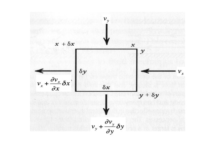
The flux of material flowing in in \(x\) direction = \( v_x \delta y\)
The flux of material flowing out in \(x\) direction = \( (v_x +\frac{\partial{v_x}}{\partial x})\delta y\)
Here we use a continuum formulation by expressing the velocity on the left-hand side of the volume in terms of the velocity on the right-hand side plus a change described by the velocity gradient field.

The net flux of material in \(x\) direction is then equal to \( (\frac{\partial{v_x}}{\partial x})\delta y\)

Similarly, the influx of material in \(y\) direction = \( v_y \delta x\)
And outflux in \(y\) direction = \( (v_y +\frac{\partial{v_y}}{\partial y})\delta x\)

The net flux of material in \(y\) direction is then equal to \( (\frac{\partial{v_y}}{\partial y})\delta x\)

If mass is conserved the net flow has to equal zero, i.e.:
Total net flow per unit area (i.e. divided by the volume area \(\delta x \delta y\)) should satisfy:

\[\frac{\partial{v_x}}{\partial x} + \frac{\partial{v_y}}{\partial y} = 0\]

General conservation of mass equation

In the expression above, you probably recognise the divergence of velocity. The continuity equation for incompressible material can be generalised to 3-D by writing it as a vector equation:

\[ \nabla \cdot \mathbf{v} = 0\]

If density is not constant then it is not sufficient to conserve volume, but full mass needs to be considered. Lets do this for an infinitesimal volume \(dV\):

\[ \frac{D\rho dV}{Dt} = 0\]

This can be written as:

\[ V \frac{D\rho}{Dt} + \rho \frac{DdV}{Dt}= 0\]

where the first term describes the changes in density and the second in volume.

Per unit volume (i.e. dividing by \(dV\)), we can write this as:

\[ \frac{D\rho}{Dt} + \rho \nabla \cdot \mathbf{v}= 0\]

In spatial description:

\[ \frac{D\rho}{Dt} = \frac{\partial \rho}{\partial t} + \mathbf{v} \cdot \nabla \rho\]

where the first term describes the changes in time of density \(\rho\) and the second term change in density by advection of density.

Putting this expression in the equation above yields the general conservation of mass equation in vector form:

\[ \frac{\partial \rho}{\partial t} + \nabla \cdot (\rho \mathbf{v})= 0\]

Conservation of Momentum

• Linear force balance = Newton’s second law, \(\mathbf{F}=m\mathbf{a}\)

• Relates force \(\mathbf{F}\) to motion, acceleration \(\mathbf{a}\). Hence also called “equation of motion”

• Conservation angular momentum assumed in symmetry of stress tensor

We can use the stress tensor to write a balance of forces in 3-D for a small volume with dimensions \(\Delta x_1\) by \(\Delta x_2\) by \(\Delta x_3\)

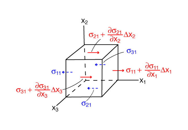
Let’s start with a balance of forces in \(x_1\) direction:

Body force = \(f_1 ~ \Delta x_1 ~ \Delta x_2 ~\Delta x_3\) , where \(f\) is force per unit volume.

The net force due to stress in \(x_1\) direction on planes with normal in \(x_1\) direction (written in continuum form, using stress gradients) equals:

\[ [(\sigma_{11} + \Delta x_1 \frac{\partial{\sigma_{11}}}{\partial x_1}) - \sigma_{11} ]\Delta x_2 ~\Delta x_3 \]

Similarly, we can write stress in \(x_1\) direction on planes with normal in \(x_2\) direction, and on planes with normal in \(x_3\) direction:

\[ [(\sigma_{21} + \Delta x_2 \frac{\partial{\sigma_{21}}}{\partial x_2}) - \sigma_{21} ]\Delta x_1 ~\Delta x_3 \]

\[ [(\sigma_{31} + \Delta x_3 \frac{\partial{\sigma_{31}}}{\partial x_3}) - \sigma_{31} ]\Delta x_1 ~\Delta x_2 \]

The total forces have to balance mass times acceleration in \(x_1\) direction:

\[ \rho \Delta x_1 ~ \Delta x_2 ~\Delta x_3 \frac{\partial^2{u_1}}{\partial t^2} \]

Dividing by the volume, gives the following force balance per unit volume:

\[ f_1 + \frac{\partial{\sigma_{11}}}{\partial x_1} + \frac{\partial{\sigma_{21}}}{\partial x_2} + \frac{\partial{\sigma_{31}}}{\partial x_3} = \rho \frac{\partial^2{u_1}}{\partial t^2} \]

General Conservation of Momentum

Generalising the previous result to all directions using index (and Einstein) notation yields:

\[ f_i + \frac{\partial{\sigma_{ji}}}{\partial x_j} = \rho \frac{\partial^2{u_i}}{\partial t^2} \]

Or in vector notation:

\[ \mathbf{f} + \nabla \cdot {\boldsymbol{\sigma}} = \rho \frac{\partial^2{\mathbf{u}}}{\partial t^2} \]

Practise

Do \(\color{blue}{\textbf{exercises 1, 2}}\)

Thermodynamics: Conservation of Energy

• First law of thermodynamics

• Preservation of energy, i.e any change in kinetic or internal energy is balanced by work done and heat used/produced

\[ \frac{D(K+U)}{Dt} = W + Q \]

Where:
\(K\) - kinetic energy
\(U\) - internal energy
\(W\) - net power input
\(Q\) - net heat input

Let’s start with the form that describes preservation of thermal energy, in 2-D

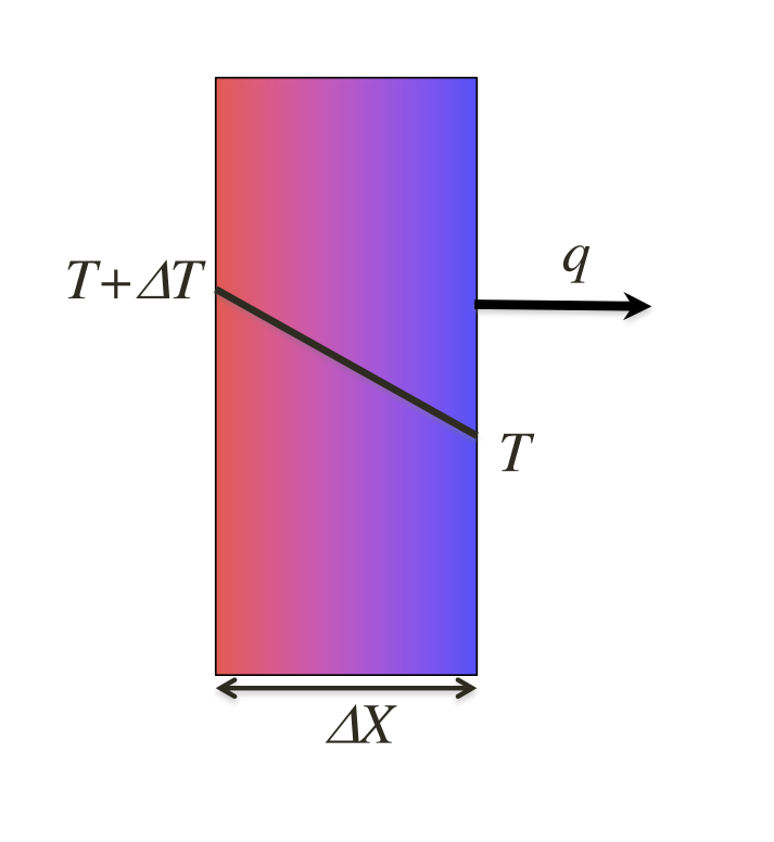
Fourier’s Law for conduction

\[q = -k \frac{dT}{dx}\]

• Heat flux, q, = heat/area = energy/time/area, unit: \(J/s/m^2\) = \(W/m^2\)

• Heat flux proportional to temperature gradient

• Minus sign because heat flows from hot to cold

• Constant of proportionality: thermal conductivity, \(k\), unit: \(W/m/K\)

1-D Steady State Conduction

• net heat flow per unit area per unit time:

\[q (x + \delta x) - q(x)\]

\[q (x + \delta x) = q(x) + \delta x \frac{dq}{dx} + ...\]

\[q(x + \delta x) - q(x) \approx \delta x \frac{dq}{dx}\]

\[\partial x \frac{dq}{dx} = \delta x \left[ \frac{d}{dx}\left(-k \frac{dT}{dx}\right) \right]\]

\[\delta x \frac{dq}{dx} = \delta x \left[-k \frac{d^2T}{dx^2} \right]\]

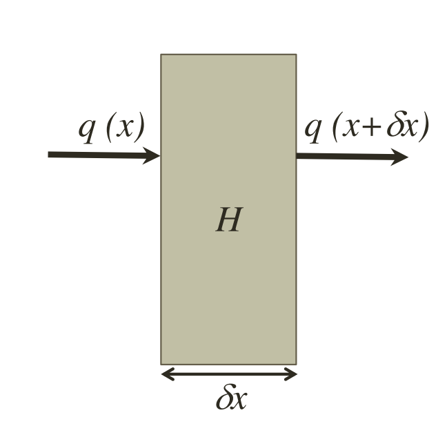
• heat produced = \(\rho H \delta x = A \delta x\)
  \(H\) - heat production rate per unit mass (\(W/kg\))
  \(A\) - heat production per unit volume (\(W/m^3\))

\[ -k \frac{d^2T}{dx^2} = \rho H = A\]

2-D Energy Equation

Spatial, constant \(\mathit{\rho}\), \(\mathit{C_P}\), k, incompressible, no heat sources

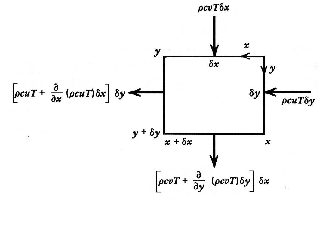
• Change in heat content:

\[\frac{\partial(\rho C_p T)}{\partial t}\delta x \delta y\]

• Advection:

\[ \left[ \frac{\partial(\rho C_p u T)}{\partial x} + \frac{\partial(\rho C_p u T)}{\partial y} \right] \delta x \delta y\]

simplifies by conservation of mass

\[ \rho C_P \left[ u \frac{\partial T}{\partial x} + v \frac{\partial T}{\partial y} \right] \delta x \delta y\]

• Conduction:

\[ -k \left( \frac{\partial^2 T}{\partial x^2} + \frac{\partial^2 T}{\partial y^2}\right) \delta x \delta y \]

Bringing it all together

\[ \rho C_P \left[\frac{\partial T}{\partial t} + u \frac{\partial T}{\partial x} + v \frac{\partial T}{\partial y} \right] = k \left( \frac{\partial^2 T}{\partial x^2} + \frac{\partial^2 T}{\partial y^2}\right)\]

\[ \rho C_P \left[\frac{\partial T}{\partial t} + \mathbf{u} \cdot \nabla T \right] = k \nabla^2 T\]

Energy Equation

• Material derivative internal heat

\[ \rho C_P \left[\frac{\partial T}{\partial t} + \mathbf{u} \cdot \nabla T \right] = \rho C_P \frac{DT}{Dt} \Rightarrow \frac{D(\rho C_P T)}{Dt} \]

Allowing for spatial variations of material parameters

• Heat input

\[ k \nabla^2 T \Rightarrow \nabla \cdot k \nabla T + A \]

\(\nabla \cdot k \nabla T\) - Conduction,
\(A\) - Internal heat production

• Work done

Change in motion (kinetic energy) and internal deformation

Net effect of \(W - \frac{DK}{Dt}\) becomes \(\mathbf{\sigma : D}\), where \(\mathbf{D}\) is strain rate

Conservation of heat

\[ D (\rho C_P T)/Dt = \nabla \cdot k \nabla T + A + \boldsymbol{\sigma}:\mathbf{D} + (\alpha T\mathbf{v} \cdot \nabla P + ....)\]

\(D (\rho C_P T)/Dt\) - Change in temperature with time
\(\nabla \cdot k \nabla T\) - Heat transfer by conduction (and radiation)
\(A\) - heat production (including latent heat)
\(\boldsymbol{\sigma}:\mathbf{D}\) - heat generated by internal deformation
\(\alpha T\mathbf{v} \cdot \nabla P\) - heat generated by adiabatic compression
\(....\) - Other heat sources, e.g. latent heat

Summary Conservation Equations

Conservation of mass
Kinematics

\[\frac{D\rho}{Dt} + \rho \nabla \cdot \mathbf{v} = 0\]

Conservation of momentum
Dynamics

Newton’s second law:
$\( \rho \frac{D\mathbf{v}}{Dt} = \nabla \cdot \boldsymbol{\sigma} + \mathbf{f} \)$

plus a condition for angular momentum: $\( \boldsymbol{\sigma} = \boldsymbol{\sigma}^T \)$

Conservation of energy
First law of thermodynamics

\[ \frac{D (\rho C_P T)}{Dt} = \nabla \cdot k \nabla T + A + \boldsymbol{\sigma} : \mathbf{D} \]

Entropy inequality
Which law is this?
Rate of entropy increase of a particle \(\geq\) entropy supply

1-D advection-diffusion solution

\[ -v_z \frac{\partial T}{\partial z} = \kappa \frac{\partial^2 T}{\partial z^2}\]

\[ \kappa = \frac{k}{\rho C_P} \]

Take \(f(z) = \frac{\partial T}{\partial z}\) and \(c = \frac{v_z}{\kappa}\)

Then \(\frac{\partial f}{\partial z} = -cf(z)\), which yields \(f(z) = f(0) e^{-cz}\)

i.e. $\(\frac{\partial T}{\partial z}(z) = A e^{-v_z z/ \kappa}\)\(, \)\(T(z) = B - \frac{A}{v_z / \kappa} e^{-v_z z/ \kappa}\)\( where \)A, B$ are integration constants

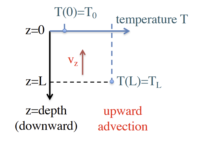
For constant temperature boundary conditions \(T(z=0) = 0\) and \(T(z=L) = T_L\) \(\Rightarrow\)
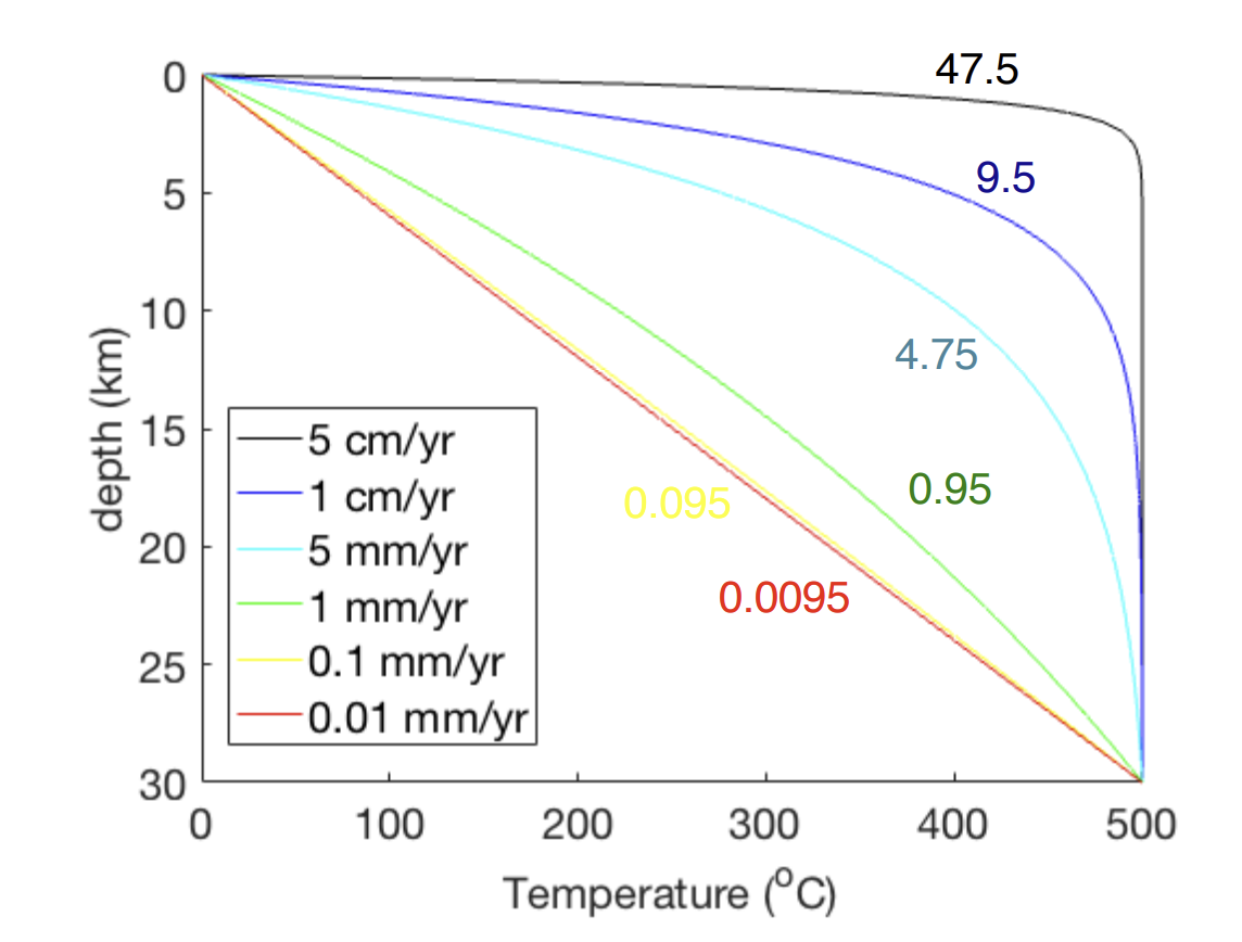
Integration gives: $\(T(z) = T_L \left[ \frac{1 - e^{-v_z z/ \kappa}}{1 - e^{-v_z L/ \kappa}}\right]\)$

What shape if diffusion dominates, if advection increases?

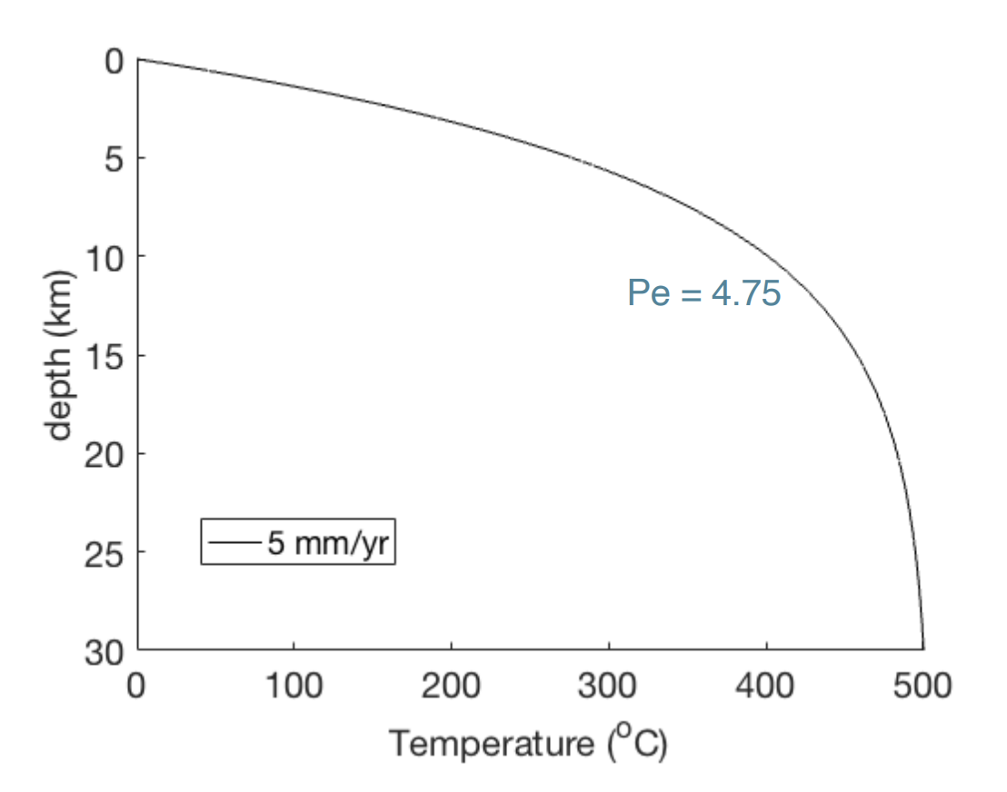
Peclet number, measure of relative importance advection/diffusion: \(Pe = \frac{v_z L}{\kappa} = \frac{[(m/s)m]}{[m^2 / s]}\)

Practise

• Use Exercise 3 to look at the shape of the solutions

• Exercise 4 for afternoon workshop