Exercises#
Learning outcomes #
At the end of this session, you should:
Know the main conservation equations used in continuum mechanics modelling and understand what different terms in these equations represent
Be able to solve conservation equations for basic analytical solutions given boundary/initial conditions.
Understand basic properties of elastic and viscous rheology and understand how the choice of rheology leads to different forms of the momentum conservation equation
Using tensor analysis to obtain relations between the main isotropic elastic parameters
Table of Contents#
# Import packages for notebook here
import numpy as np
import matplotlib.pyplot as plt

%matplotlib inline
Do not alter this cell. LaTeX commands for frequently used terms.
Continuum mechanics equations#
Continuum mechanical modelling involves solving one or more of a set of equations that capture:
Kinematics - describing deformation and velocity without considering forces
Dynamics - describing the balance of forces, i.e., conservation of linear and angular momentum
Thermodynamics - describing the relation between temperature, heatflux, stress, entropy
Constitutive equations - describing how material properties vary as a function of temperature, pressure, stress,…
The main set of equations are:
Conservation of mass
Conservation of momentum (Newton’s second law for linear momentum)
Conservation of energy (First law of thermodynamics)
Some problems can be addressed by solving one of these equations alone (e.g. the conservation of energy to solve how heat transfers conductively through an object heated from one side), or a coupled set of equations (e.g. flow of a hot fluid through a porous medium by jointly solving conservation of mass, momentum and energy).
If material properties vary with any of the primary parameters, then additional equations, describing for example viscosity or thermal conductivity, need to be added.
The continuity equation (conservation of mass)#
The continuity equation captures the requirement that no mass is lost during deformation or flow.
As discussed in the lecture, if material is incompressible, i.e. its density does not change during flow or deformation, this equation reduces to the form:
If the density changes in time and/or space, additional terms need to be included, yielding the following equation:
in spatial description:
or in material description:
Exercise 1#
Given the following 3D velocity field,
where \(k\) is a constant, find the density of a material particle as a function of time; i.e., derive \(\rho(t)\).
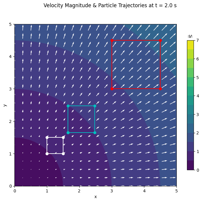
Going back to the (2D version of) the same velocity field from the first example, plotting how the shapes change size as they move through the flow, visualises how density evolves.
# Make a position grid fine enough to represent velocities as a smooth field.
def init_grid(Lx=10., dx=None, Ly=10., dy=None):

    # Use 100 grid points if dx not specified
    if dx is None:
        dx = Lx/100.
    if dy is None:
        dy = Ly/100.

    # Construct the grid
    nx = int(Lx/dx)
    xx = np.linspace(0, Lx, nx)
    ny = int(Lx/dx)
    yy = np.linspace(0, Ly, ny)
    X, Y = np.meshgrid(xx, yy)

    return X, Y

# Define the initial positions of a set of tracer particles to show motion/deformation
# Construct two 2D numpy arrays, one for each coordinate direction. The first dimension
# is the particle number; the second is the time level. . .
def tracers(p0=[[0.5, 0.5], [1.5, 0.5], [1.5, 1.5], [0.5, 1.5], [0.5, 0.5]], nt=11):

    # Create arrays
    px = np.zeros((len(p0), nt))
    py = np.zeros_like(px)

    # Initialise with specified initial coordinates.
    for p, i in zip(p0, range(len(p0))):
        px[i,:] = p[0]
        py[i,:] = p[1]

    return px, py
# Define a spatial grid with 100 x 100 points. . .
X, Y = init_grid(Lx=5., Ly=5.)

# Choose a time discretisation fine enough for integrating particle paths
# with enough precision to reproduce the analytical solution discussed in the lecture.
dt = 0.05
tt = np.arange(0, 2 + dt, dt)
nt = tt.size

# Define five tracers in a square to track shape change
px, py = tracers(p0=[[1., 1.], [1.5, 1.], [1.5, 1.5], [1., 1.5], [1., 1.]], nt=nt)
# Define the spatial description of a 2D velocity field as a function of x, y and time.
# You can modify this to consider different spatial velocity functions. . .
k=1
def velocity_spatial(x, y, t, k=1):
    return k*x/(1+k*t), k*y/(1+k*t)

def material_position(xi_x, xi_y, t, k=1):
    return (1+k*t)*xi_x, (1+k*t)*xi_y
# Define velocity field at last time step
vx, vy = velocity_spatial(X, Y, tt[nt-1], k=k)
vmag = np.sqrt(vx**2 + vy**2)

# Define the particle position using our analytical function
for it in range(1,nt):
    px[:, it], py[:, it] = material_position(px[:, 0], py[:, 0], tt[it])

# Plot the velocity field at time zero
plt.figure(figsize=(9,7))
plt.subplot(aspect='equal')
plt.suptitle("Velocity Magnitude & Particle Trajectories at t = %1.1f s" % tt[-1])
plt.xlabel('x')
plt.ylabel('y')

# Define a sensible fixed colorscale
cc = np.arange(0, 7.5, 0.5)
cl = np.arange(0, 8, 1)

# Contour plot of velocity magnitude
c = plt.contourf(X, Y, vmag, cc)
cbar = plt.colorbar(c, shrink=0.8, ticks=cl)
cbar.ax.set_title("$\\left| v \\right|$")

# Quiver plot of velocity vector field
plt.quiver(X[::5,::5], Y[::5,::5], vx[::5,::5], vy[::5,::5], color='w')

# Plot tracer square at three time levels; beginning, one-third time and end time.
plt.plot(px[:, 0], py[:, 0], 'wo-')
plt.plot(px[:, int(nt/3)], py[:, int(nt/3)], 'co-')
plt.plot(px[:,-1], py[:,-1], 'ro-')

plt.show()
The equation of motion and force equilibrium#
In the lecture we saw how taking a force balance acting on an infinitesimal cube in a continuum results in a partial differential equation that describes the conservation of momentum,
or
The term on the left-hand side is the mass (per unit volume) times the acceleration; the terms on the right-hand side are therefore the sum of the forces (per unit mass) acting on the body, which for each coordinate direction include the net body force (per unit mass) \(\vector{f}\) and the sum of the stress gradients \(\nabla\cdot\tensor{\sigma}\) acting in that direction.
This implies that if the continuum is in equilibrium at a point (i.e., no acceleration), the body force and stress gradients must be in exact balance in each direction.
If there is no body force then the sum of the stress gradients in each coordinate direction must be zero.
Exercise 2#
Consider the following stress distribution:
where \(\sigma_{12}\) is a linear function of \(x_1\) and \(x_2\).
Find \(\sigma_{12}\) given that the stress vector on plane \(x_1 = 1\) is given by:
and that the stress distribution is in equilibrium with zero body force.
Conservation of Energy#
The general form of the conservation of energy equation that we considered in the lecture is:
where, from left to right, the different terms represent:
change in temperature with time
heat transfer by conduction (and radiation)
heat production (including latent heat)
heat generated by internal deformation
1D Advection-Diffusion#
In the lecture, we saw how the conservation of energy equation simplifies to the 1-D steady-state advection-diffusion equation in the absence of spatial variation in material parameters, internal deformation and heat production \(A\):
where:
\(T\) is temperature (in \(^{\circ}\)C)
\(z\) is depth (in m)
\(\kappa = k/(\rho C_p)\) is thermal diffusivity (in m\(^2\)/s)
\(v_z\) vertical velocity (in m/s)
Use the code below to calculate and plot analytical solutions to the 1-D steady state advection-diffusion equation for the transport of heat, with constant temperature boundary conditions at \(z=0\) and \(z=L\).
Exercise 3#
Use the code below to calculate and plot analytical solutions to the 1-D steady state advection-diffusion equation for the transport of heat, with constant temperature boundary conditions at \(z=0\) and \(z=L\).
Step 1: Set parameter values. In the example, values applicable to Earth’s crust are chosen, but feel free to try others appropriate for a different problem
# Thermal diffusivity for rocks (m^2/s)
kap=1e-6

# Depth range from surface to 30 km depth, in small steps
dz = 0.2e3
zz = np.arange(0, 30e3, dz)
nz = zz.size
LL = np.amax(zz)

# A range of vertical advection velocity values
yr2sec=3600.*24.*365.25
nv = 6
vz = np.zeros(nv)
# 5 cm/yr
vz[0]=5e-2/yr2sec
# 1 cm/yr
vz[1]=1e-2/yr2sec
# 5 mm/yr
vz[2]=5e-3/yr2sec
# 1 mm/yr
vz[3]=1e-3/yr2sec
# 0.1 mm/yr
vz[4]=1e-4/yr2sec
# 0.01 mm/yr
vz[5]=1e-5/yr2sec
# 5 mm/yr
vzcm = vz*1e2*yr2sec

# Boundary conditions:
# constant surface temperature and temperature at base of the domain
T0=0            # surface temperature of 0 oC
TL=500          # temperature at zmax=L of 500 oC
Step 2: Compute and plot temperature solutions for the range of advection velocities
# Initialise set up for figure
tempfig, ax= plt.subplots(1)
tempfig.suptitle("Temperatures vs Depth")
linecol=['k-','b-','c-','g-','y-','r-','m']
ax.set_ylim(LL, 0)
plt.xlabel("Temperature $^{\circ}$C")
plt.ylabel("Depth (m)")

# Determine temperatures for each advection velocities
# and add line to figure
for iv in range(nv):
    # initialise temperature
    Tzz=np.zeros(nz)
    # calculate temperature for this vz
    cc=-1.*vz[iv]/kap
    prefac=TL/(1.-np.exp(cc*LL))
    Tzz=prefac*(1.-np.exp(cc*zz))
    plt.plot(Tzz,zz,linecol[iv],label=str("{:.2f}".format(vzcm[iv])))
plt.legend(title='vz (cm/yr)')
plt.show()
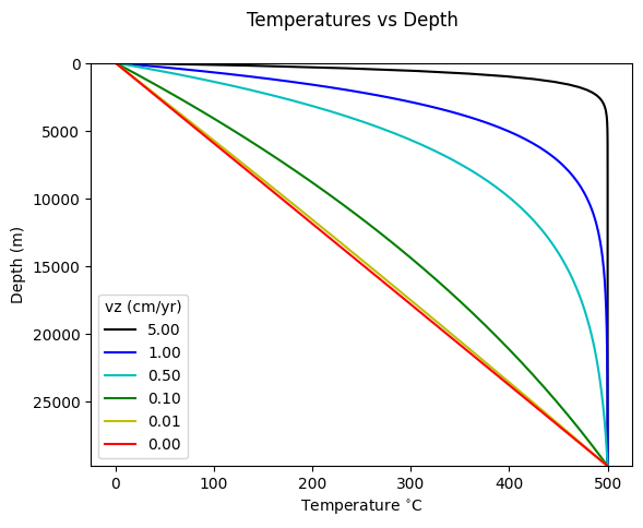
The relative importance of heat advection and heat conduction determines the shape of the temperature-depth profiles. The dimensionless parameter that captures this relative importance is called the Peclet number, \(Pe\).
where \(v_z\) is vertical velocity, \(L\) is a length scale characteristic of the problem (in this case the depth scale), and \(\kappa\) is thermal diffusivity.
In many physical problems, there are dimensionless numbers that characterise the type of solution. This will be discussed further in the next lecture.
Step 3: Calculate Peclet numbers for these solutions. What do large/small \(Pe\) indicate?
Pecletno=vz*LL/kap
with np.printoptions(precision=3, suppress=True):
    print('Advection velocity: ',vz*100*yr2sec, 'cm/yr')
    print('Peclet number: ',Pecletno)
Advection velocity:  [5.    1.    0.5   0.1   0.01  0.001] cm/yr
Peclet number:  [47.215  9.443  4.722  0.944  0.094  0.009]
(Optional)
Things you could try yourself:
Evaluate how the profile and Peclet number change with advection velocity. At what velocity does the solution become essentially conductive?
Add a heat production term (e.g. A = 0.4 \(\mu\)W/m\(^3\))
Find solution for boundary conditions: \(T\)(\(z\)=0)=0 \(^{\circ}\)C and \(\partial T/\partial z\)(\(z\)=0)=20\(^{\circ}\)C/km and plot for different values of \(v_z\).
Exercise 4#
(a) Write down the energy equation for a 1-D steady state problem with internal heat production, but without any contribution of strain or flow.
(b) Solve this equation for a layer with constant material properties, with a fixed temperature on the bottom and an insulating top:
(c) Plot the solution for the following parameter values: \(T_0 = 0^\circ\)C, \(k = 80\) Wm\(^{-1}\)K\(^{-1}\), \(A = 200\) Wm\(^{-3}\), \(h = 2\) m.
(Optional)
(d) You could vary the values of \(A\) and \(k\) to get more insight in the relative effects of heat production and conductivity on the temperature profile.
Conservation of Momentum: Hookean Elasticity#
In the lecture, we saw how combining the conservation of momentum equation with the constitutive equation for an elastic material leads to the elastic wave equation.
For an isotropic Hookean solid, the constitutive equation only involves two elastic parameters, taking the following form when cast in terms of the two Lamé constants: $\(\sigma_{ij}=\lambda \epsilon_{kk} \delta_{ij} + 2 \mu \epsilon_{ij}\)$
(Optional)
Writing out the missing steps in the derivation in the lecture slides is a good practise of tensor and index notation skills
Remembering that the conservation of momentum, in index notation is: $\(\rho\frac{\partial^2 u_{i}}{\partial t^2} = f_{i} + \frac{\partial{\sigma_{ji}}}{\partial{x_{j}}}\)$
With the above elastic constitutive equation, the divergence of the stress tensor is: $$ \frac{\partial{\sigma_{ji}}}{\partial{x_{j}}} = \lambda \frac{\partial{(\partial{u_{k}}/\partial{x_{k}})}}{\partial{x_{i}}}
\mu \frac{\partial^2 u_i}{\partial
\mu \frac{\partial{(\partial{u_{j}}/\partial{x_{j}})}}{\partial{x_{i}}}$$
Or in vector form $\(\nabla\cdot\vector{\sigma}=(\lambda+\mu)\nabla(\nabla\cdot\vector{u})+\mu\nabla^2\vector{u}\)$
Using the relation: $\(\nabla^2\vector{u}=\nabla(\nabla\cdot\vector{u})-\nabla\times\nabla\times\vector{u}\)$
This yields the following elastic wave equation:
The term with \(\nabla\cdot\vector{u}\) describes changes in volume due to the displacement field and is related to compressional waves, while the term with \(\nabla\times\vector{u}\) describes the rotational component of the displacement field and is related to shear waves.
Exercise 5#
Two alternative elastic parameters often used are the bulk modulus \(K\) and shear modulus \(G\). These two moduli are linked, respectively, to isotropic stress (i.e. pressure \(p\)) and strain (\(\theta\)): $\( -p = \frac{\sigma_{kk}}{3} = K \epsilon_{kk} = K \theta \)$
and deviatoric stress \(\sigma'_{ij}\) and strain \(\epsilon'_{ij}\): $\( \sigma'_{ij} = \sigma_{ij} + p \delta_{ij} = 2 G \epsilon'_{ij} \)$
Derive the expressions relating \(K\) and \(G\) to the Lamé constants \(\lambda\) and \(\mu\)
Exercise 6 (Advanced)#
(a) Show that for an isotropic Hookean solid, the principal directions of stress and strain coincide.
(b) Find a relation between the principal values of stress and strain using the two Lamé parameters.
(c) For the same Hookean solid, express the elastic Young’s modulus \(E\) and Poisson’s ratio \(\nu\), which are often used in engineering, in terms of the Lamé parameters \(\lambda\) and \(\mu\).
The two engineering moduli are defined for a uniaxial state of stress, where \(\sigma_1 \ne 0\) and \(\sigma_2 = \sigma_3 = 0\), a useful system for experimentally determining the elastic parameters. This stress leads to a maximum strain \(\epsilon_1\) in the direction of the applied stress and uniform strain in perpendicular direction, \(\epsilon_2 = \epsilon_3\).
The moduli are then defined as: